Page 277 - Computational Statistics Handbook with MATLAB

266 Computational Statistics Handbook with MATLAB

FREEDMAN-DIACONIS RULE

⁄
ˆ * – 13
hHist = 2 × IQR × n .
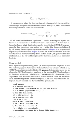
It turns out that when the data are skewed or heavy-tailed, the bin widths
are too large using the Normal Reference Rule. Scott [1979, 1992] derived the
following correction factor for skewed data:

⁄
2 13 σ
skewness factor Hist = ------------------------------------------------------------------ . (8.13)
⁄
⁄
2
5σ ⁄ 4 2 13 σ 2 12
e ( σ + 2) ( e – 1)
The bin width obtained from Equation 8.12 should be multiplied by this fac-
tor when there is evidence that the data come from a skewed distribution. A
factor for heavy-tailed distributions can be found in Scott [1992]. If one sus-
pects the data come from a skewed or heavy-tailed distribution, as indicated
by calculating the corresponding sample statistics (Chapter 3) or by graphical
exploratory data analysis (Chapter 5), then the Normal Reference Rule bin
widths should be multiplied by these factors. Scott [1992] shows that the
modification to the bin widths is greater for skewness and is not so critical for
kurtosis.

Example 8.2
Data representing the waiting times (in minutes) between eruptions of the
Old Faithful geyser at Yellowstone National Park were collected [Hand, et al,
1994]. These data are contained in the file geyser. In this example, we use an
alternative MATLAB function (available in the standard MATLAB package)
for finding a histogram, called histc. This takes the bin edges as one of the
arguments. This is in contrast to the hist function that takes the bin centers
as an optional argument. The following MATLAB code will construct a his-
togram density estimate for the Old Faithful geyser data.

load geyser
n = length(geyser);
% Use Normal Reference Rule for bin width.
h = 3.5*std(geyser)*n^(-1/3);
% Get the bin mesh.
t0 = min(geyser)-1;
tm = max(geyser)+1;
rng = tm - t0;
nbin = ceil(rng/h);
bins = t0:h:(nbin*h + t0);
% Get the bin counts vk.
vk = histc(geyser,bins);
% Normalize to make it a bona fide density.

© 2002 by Chapman & Hall/CRC