Page 278 - Computational Statistics Handbook with MATLAB

Chapter 8: Probability Density Estimation 267

% We do not need the last count in fhat.
fhat(end) = [];
fhat = vk/(n*h);
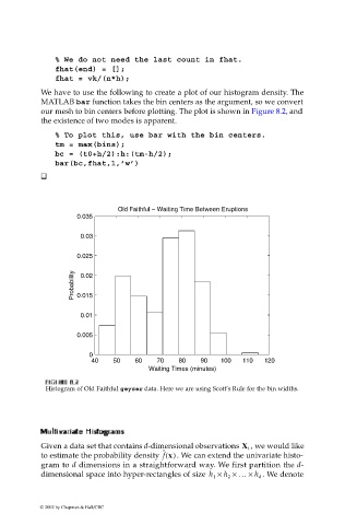
We have to use the following to create a plot of our histogram density. The
MATLAB bar function takes the bin centers as the argument, so we convert
our mesh to bin centers before plotting. The plot is shown in Figure 8.2, and
the existence of two modes is apparent.

% To plot this, use bar with the bin centers.
tm = max(bins);
bc = (t0+h/2):h:(tm-h/2);
bar(bc,fhat,1,’w’)

Old Faithful − Waiting Time Between Eruptions
0.035

0.03

0.025

Probability 0.015
0.02

0.01

0.005

0
40 50 60 70 80 90 100 110 120
Waiting Times (minutes)

IG
FI F U URE G 8. RE 8. 2 2
F F II GU RE RE 8. 8. 2
2
GU
Histogram of Old Faithful geyser data. Here we are using Scott’s Rule for the bin widths.

ooggrr aamm ss
ee
Multi MultMult Mult ivvar vvarar ar i iaat aatt teeHHi HHii isst sstt toog gr raamms s
ii
ii
, we would like
Given a data set that contains d-dimensional observations X i
ˆ
to estimate the probability density f x() . We can extend the univariate histo-
gram to d dimensions in a straightforward way. We first partition the d-
dimensional space into hyper-rectangles of size h 1 × h 2 × … × h d . We denote
© 2002 by Chapman & Hall/CRC