Page 296 - Computational Statistics Handbook with MATLAB

Chapter 8: Probability Density Estimation 285

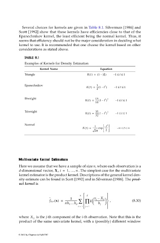
Several choices for kernels are given in Table 8.1. Silverman [1986] and
Scott [1992] show that these kernels have efficiencies close to that of the
Epanechnikov kernel, the least efficient being the normal kernel. Thus, it
seems that efficiency should not be the major consideration in deciding what
kernel to use. It is recommended that one choose the kernel based on other
considerations as stated above.

T
T
T A BL LE L 8.1 E E 8.1
TA
AB
A
B
L
B
8.1
8.1
E
Examples of Kernels for Density Estimation
Kernel Name Equation
t
Triangle Kt() = ( 1 – t ) – 1 ≤≤ 1
Epanechnikov 3
2
-
t
Kt() = -- 1 –( t ) – 1 ≤≤ 1
4
Biweight 15 2 2
-
t
Kt() = ----- 1 –( t ) – 1 ≤≤ 1
16
Triweight 35 2 3
t
-
Kt() = ----- 1 –( t ) – 1 ≤≤ 1
32
Normal  t – 
2
1
Kt() = ---------- exp  -------  – ∞ << ∞
t
2π  2 
E
Est
r
e
v
r
K
eK
tt
Ke
e
ne
n
e
Mult Mult Mult Mult i ii iv var v ar i ar ar ii ia at a a te e K er e rn n el e ll lE E st i st st mator i ii mator mator mator s s s s
Here we assume that we have a sample of size n, where each observation is a
d-dimensional vector, X i i, = 1 … n . The simplest case for the multivariate
,
,
kernel estimator is the product kernel. Descriptions of the general kernel den-
sity estimate can be found in Scott [1992] and in Silverman [1986]. The prod-
uct kernel is
 
n d
-----------------
ˆ 1   x j – X ij 
f Ker x() = -------------------- ∑  ∏ K    , (8.30)
nh 1 …h d  h j 
i = 1  j = 1 
where X ij is the j-th component of the i-th observation. Note that this is the
product of the same univariate kernel, with a (possibly) different window
© 2002 by Chapman & Hall/CRC