Page 301 - Computational Statistics Handbook with MATLAB

290 Computational Statistics Handbook with MATLAB

,
(
2
where φ x µσ ) represents the normal probability density function at x. We
;
see from the model that we have three terms or component densities, cen-
tered at -3, 0, and 2. The mixing coefficient or weight for the first two terms
are 0.3 leaving a weight of 0.4 for the last term. The following MATLAB code
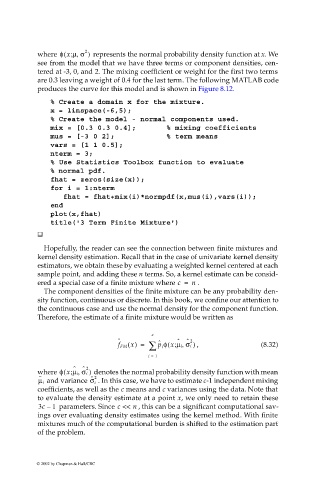
produces the curve for this model and is shown in Figure 8.12.
% Create a domain x for the mixture.
x = linspace(-6,5);
% Create the model - normal components used.
mix = [0.3 0.3 0.4]; % mixing coefficients
mus = [-3 0 2]; % term means
vars = [1 1 0.5];
nterm = 3;
% Use Statistics Toolbox function to evaluate
% normal pdf.
fhat = zeros(size(x));
for i = 1:nterm
fhat = fhat+mix(i)*normpdf(x,mus(i),vars(i));
end
plot(x,fhat)
title('3 Term Finite Mixture')

Hopefully, the reader can see the connection between finite mixtures and
kernel density estimation. Recall that in the case of univariate kernel density
estimators, we obtain these by evaluating a weighted kernel centered at each
sample point, and adding these n terms. So, a kernel estimate can be consid-
ered a special case of a finite mixture where c = n .
The component densities of the finite mixture can be any probability den-
sity function, continuous or discrete. In this book, we confine our attention to
the continuous case and use the normal density for the component function.
Therefore, the estimate of a finite mixture would be written as

c
ˆ ˆ ˆ ˆ 2
,
(
;
f FM x() = ∑ p i φ x µ i σ i , ) (8.32)
i = 1
ˆ ˆ 2
(
,
where φ x µ i σ i ) denotes the normal probability density function with mean
;
ˆ ˆ 2
µ i and variance σ i . In this case, we have to estimate c-1 independent mixing
coefficients, as well as the c means and c variances using the data. Note that
to evaluate the density estimate at a point x, we only need to retain these
3c – 1 parameters. Since c << n , this can be a significant computational sav-
ings over evaluating density estimates using the kernel method. With finite
mixtures much of the computational burden is shifted to the estimation part
of the problem.

© 2002 by Chapman & Hall/CRC