Page 303 - Computational Statistics Handbook with MATLAB

292 Computational Statistics Handbook with MATLAB

dF Plot for Univariate Finite Mixture

0.9
0.8
0.7
Mixing Coefficients 0.5
0.6

0.4
0.3
0.2
0.1
0
−5 −4 −3 −2 −1 0 1 2 3 4 5
Means

8.13
8.13
II
GU
GU
F FI F F IG URE G 8.13 RE RE RE 8.13
U
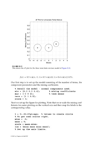
This shows the dF plot for the three term finite mixture model of Figure 8.12.
(
,
,
(
(
,
;
–
;
f x() = 0.3 × φ x 31) + 0.3 × φ x 01) + 0.4 × φ x 20.5 . )
;
Our first step is to set up the model consisting of the number of terms, the
component parameters and the mixing coefficients.
% Recall the model - normal components used.
mix = [0.3 0.3 0.4]; % mixing coefficients
mus = [-3 0 2]; % term means
vars = [1 1 0.5];
nterm = 3;
Next we set up the figure for plotting. Note that we re-scale the mixing coef-
ficients for easier plotting on the vertical axis and then map the labels to the
corresponding value.
t = 0:.05:2*pi+eps; % values to create circle
% To get some scales right.
minx = -5;
maxx = 5;
scale = maxx-minx;
lim = [minx maxx minx maxx];
% Set up the axis limits.

© 2002 by Chapman & Hall/CRC