Page 308 - Computational Statistics Handbook with MATLAB

Chapter 8: Probability Density Estimation 297

Mix Coefs

.5 1

2
1
Mu z 0

−1

−2
6
4
2 4
0 0 2
−2 −2
Mu Mu
y x
GU
II
8.15
8.15
GU
F F FI F IG URE G 8.15 RE RE RE 8.15
U
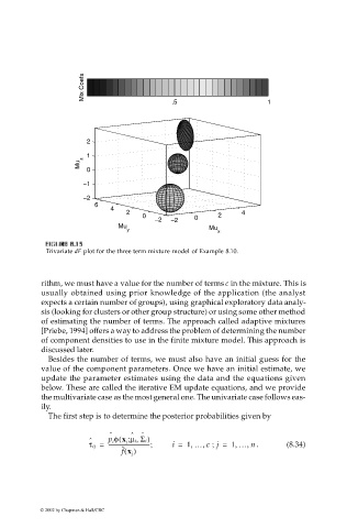
Trivariate dF plot for the three term mixture model of Example 8.10.
rithm, we must have a value for the number of terms c in the mixture. This is
usually obtained using prior knowledge of the application (the analyst
expects a certain number of groups), using graphical exploratory data analy-
sis (looking for clusters or other group structure) or using some other method
of estimating the number of terms. The approach called adaptive mixtures
[Priebe, 1994] offers a way to address the problem of determining the number
of component densities to use in the finite mixture model. This approach is
discussed later.
Besides the number of terms, we must also have an initial guess for the
value of the component parameters. Once we have an initial estimate, we
update the parameter estimates using the data and the equations given
below. These are called the iterative EM update equations, and we provide
the multivariate case as the most general one. The univariate case follows eas-
ily.
The first step is to determine the posterior probabilities given by

ˆ ˆ
ˆ
,
(
;
ˆ p i φ x j µ i Σ i)
,
,
,
,
τ ij = -------------------------------; i = 1 … c ; j = 1 … n . (8.34)
ˆ ()
f x j
© 2002 by Chapman & Hall/CRC