Page 310 - Computational Statistics Handbook with MATLAB

Chapter 8: Probability Density Estimation 299

2. Determine an initial guess at the component parameters. These are
the mixing coefficients, means and covariance matrices for each
normal density.
3. For each data point x j , calculate the posterior probability using
Equation 8.34.
4. Update the mixing coefficients, the means and the covariance ma-
trices for the individual components using Equations 8.36 through
8.38.
5. Repeat steps 3 through 4 until the estimates converge.

Typically, step 5 is implemented by continuing the iteration until the changes
in the estimates at each iteration are less than some pre-set tolerance. Note
that with the iterative EM algorithm, we need to use the entire data set to
simultaneously update the parameter estimates. This imposes a high compu-
tational load when dealing with massive data sets.

Example 8.11
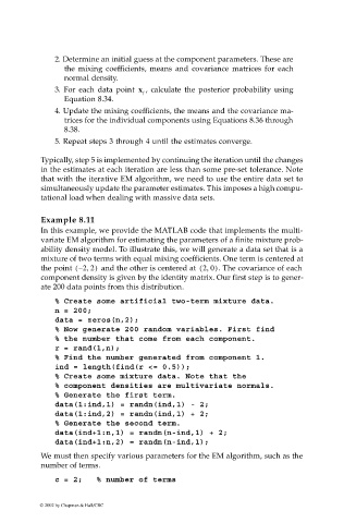
In this example, we provide the MATLAB code that implements the multi-
variate EM algorithm for estimating the parameters of a finite mixture prob-
ability density model. To illustrate this, we will generate a data set that is a
mixture of two terms with equal mixing coefficients. One term is centered at
,
the point –( 2 2) and the other is centered at 20,( ) . The covariance of each
component density is given by the identity matrix. Our first step is to gener-
ate 200 data points from this distribution.

% Create some artificial two-term mixture data.
n = 200;
data = zeros(n,2);
% Now generate 200 random variables. First find
% the number that come from each component.
r = rand(1,n);
% Find the number generated from component 1.
ind = length(find(r <= 0.5));
% Create some mixture data. Note that the
% component densities are multivariate normals.
% Generate the first term.
data(1:ind,1) = randn(ind,1) - 2;
data(1:ind,2) = randn(ind,1) + 2;
% Generate the second term.
data(ind+1:n,1) = randn(n-ind,1) + 2;
data(ind+1:n,2) = randn(n-ind,1);
We must then specify various parameters for the EM algorithm, such as the
number of terms.
c = 2; % number of terms

© 2002 by Chapman & Hall/CRC