Page 313 - Computational Statistics Handbook with MATLAB

302 Computational Statistics Handbook with MATLAB

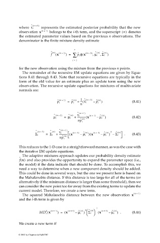
ˆ n +( 1)
where τ i represents the estimated posterior probability that the new
1
observation x ( n + ) belongs to the i-th term, and the superscript n() denotes
the estimated parameter values based on the previous n observations. The
denominator is the finite mixture density estimate

c
ˆ n() x ( n + 1) ) = ∑ p i φ x ( n + 1) ˆ n() ˆ n()
f (
(
; µ i ,
Σ i )
ˆ
i = 1
for the new observation using the mixture from the previous n points.
The remainder of the recursive EM update equations are given by Equa-
tions 8.41 through 8.43. Note that recursive equations are typically in the
form of the old value for an estimate plus an update term using the new
observation. The recursive update equations for mixtures of multivariate
normals are:

n ()
ˆ ( n + ) ˆ n () 1 ˆ n +( 1) p i )
1
(
ˆ
p i = p i + --- τ i – (8.41)
n
ˆ n +( 1)
n ()
ˆ n +( 1) ˆ n() ------------- x ( ( n + 1) µ i )
ˆ
τ i
µ i = µ i + n () – (8.42)
ˆ
np i
ˆ n +(
ˆ n +( 1) ˆ n() τ i 1) ( n + 1) n () ( n + 1) n () T ˆ n()
ˆ
ˆ
= Σ i + ------------- x ( – µ i ) x( – µ i ) – . (8.43)
Σ i n () Σ i
ˆ
np i
This reduces to the 1-D case in a straightforward manner, as was the case with
the iterative EM update equations.
The adaptive mixtures approach updates our probability density estimate
ˆ f x() and also provides the opportunity to expand the parameter space (i.e.,
the model) if the data indicate that should be done. To accomplish this, we
need a way to determine when a new component density should be added.
This could be done in several ways, but the one we present here is based on
the Mahalanobis distance. If this distance is too large for all of the terms (or
alternatively if the minimum distance is larger than some threshold), then we
can consider the new point too far away from the existing terms to update the
current model. Therefore, we create a new term.
( n + 1)
The squared Mahalanobis distance between the new observation x
and the i-th term is given by
– 1

n ()
ˆ n()
n () T
MD i x ( ( n + ) ) = x ( ( n + 1) – µ i ) Σ i   x ( ( n + 1) – µ i ) . (8.44)
ˆ
ˆ
2
1

We create a new term if
© 2002 by Chapman & Hall/CRC