Page 69 - Computational Statistics Handbook with MATLAB

Chapter 3: Sampling Concepts 55

µ
3
γ = --------- , (3.5)
1 32
⁄
µ 2
and
µ
γ = ----- 4 . (3.6)
2
2
µ 2
Substituting the sample moments for the population moments in Equations
3.5 and 3.6, we have

n
--- ∑ ( X i – X) 3
1
n
ˆ i = 1
γ 1 = ----------------------------------------------- , (3.7)
⁄
 1 n 2 32
 --- ∑ ( X i – X ) 
 n i = 1 
and

n
1 ( X) 4
--- ∑ X i –
n
ˆ i = 1
γ 2 = --------------------------------------------- . (3.8)
 n  2
2
 1 ∑ ( X i – X ) 
---
 n 
 i = 1 
ˆ is an estimate
We are using the ‘hat’ notation to denote an estimate. Thus, γ 1
. The following example shows how to use MATLAB to obtain the sam-
for γ 1
ple coefficient of skewness and sample coefficient of kurtosis.

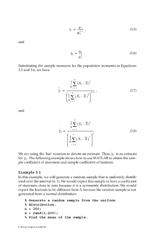
Example 3.1
In this example, we will generate a random sample that is uniformly distrib-
uted over the interval (0, 1). We would expect this sample to have a coefficient
of skewness close to zero because it is a symmetric distribution. We would
expect the kurtosis to be different from 3, because the random sample is not
generated from a normal distribution.

% Generate a random sample from the uniform
% distribution.
n = 200;
x = rand(1,200);
% Find the mean of the sample.

© 2002 by Chapman & Hall/CRC