Page 71 - Computational Statistics Handbook with MATLAB

Chapter 3: Sampling Concepts 57

independent, then ρ XY, = 0 . Note that the converse of this statement does
not necessarily hold.
There are statistics that can be used to estimate these quantities. Let’s say
,
(
we have a random sample of size n denoted as X 1 Y 1 ) … X n Y n ), ( , , . The
sample covariance is typically calculated using the following statistic
n
ˆ 1
(
σ XY, = ------------ ∑ ( X – X) Y – Y) . (3.11)
i
i
n – 1
i = 1
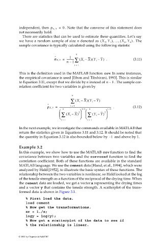
This is the definition used in the MATLAB function cov. In some instances,
the empirical covariance is used [Efron and Tibshirani, 1993]. This is similar
to Equation 3.11, except that we divide by n instead of n – 1 . The sample cor-
relation coefficient for two variables is given by

n
∑ ( X i – X) Y i – Y)
(
ˆ i = 1
ρ XY, = ------------------------------------------------------------------------------------- . (3.12)
⁄
⁄
 n 2  12  n 2  12
 ∑ ( X – X)   ∑ ( Y – Y) 
i
i
   
i = 1 i = 1
In the next example, we investigate the commands available in MATLAB that
return the statistics given in Equations 3.11 and 3.12. It should be noted that
the quantity in Equation 3.12 is also bounded below by 1– and above by 1.

Example 3.2
In this example, we show how to use the MATLAB cov function to find the
covariance between two variables and the corrcoef function to find the
correlation coefficient. Both of these functions are available in the standard
MATLAB language. We use the cement data [Hand, et al., 1994], which were
analyzed by Hald [1952], to illustrate the basic syntax of these functions. The
relationship between the two variables is nonlinear, so Hald looked at the log
of the tensile strength as a function of the reciprocal of the drying time. When
the cement data are loaded, we get a vector x representing the drying times
and a vector y that contains the tensile strength. A scatterplot of the trans-
formed data is shown in Figure 3.1.
% First load the data.
load cement
% Now get the transformations.
xr = 1./x;
logy = log(y);
% Now get a scatterplot of the data to see if
% the relationship is linear.

© 2002 by Chapman & Hall/CRC