Page 73 - Computational Statistics Handbook with MATLAB

Chapter 3: Sampling Concepts 59

4

3.8

3.6
Log of Tensile Strength 3.4 3

3.2

2.8
2.6

2.4
0 0.2 0.4 0.6 0.8 1
Reciprocal of Drying Time
FI F IG URE G 3. RE 3. 1 1
U
F F II GU RE RE 3. 3. 1
GU
1
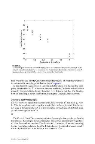
This scatterplot shows the observed drying times and corresponding tensile strength of the
cement. Since the relationship is nonlinear, the variables are transformed as shown here. A
linear relationship seems to be a reasonable model for these data.
then we must use Monte Carlo simulation techniques or bootstrap methods
to estimate the sampling distribution (see Chapter 6).
To illustrate the concept of a sampling distribution, we discuss the sam-
pling distribution for , where the random variable X follows a distribution
X
given by the probability density function f x() . It turns out that the distribu-
tion for the sample mean can be found using the Central Limit Theorem.

CENTRAL LIMIT THEOREM
Let f x() represent a probability density with finite variance σ 2 and mean . Also,
µ
X
let be the sample mean for a random sample of size n drawn from this distribution.
X
For large n, the distribution of is approximately normally distributed with mean
µ and variance given by σ ⁄ . n
2

The Central Limit Theorem states that as the sample size gets large, the dis-
tribution of the sample mean approaches the normal distribution regardless
of how the random variable X is distributed. However, if we are sampling
from a normal population, then the distribution of the sample mean is exactly
2
µ
normally distributed with mean and variance σ ⁄ n .

© 2002 by Chapman & Hall/CRC