Page 84 - Computational Statistics Handbook with MATLAB

70 Computational Statistics Handbook with MATLAB

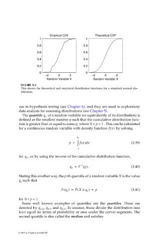
Empirical CDF Theoretical CDF
1 1
0.8 0.8

0.6 0.6
0.4 0.4
0.2 0.2

0 0
−2 0 2 −2 0 2
Random Variable X Random Variable X

F F F FI II U URE GU 3. RE RE RE 3. 3. 3. 2 2
IG
GU
G
2
2
This shows the theoretical and empirical distribution functions for a standard normal dis-
tribution.
ues in hypothesis testing (see Chapter 6), and they are used in exploratory
data analysis for assessing distributions (see Chapter 5).
of a random variable (or equivalently of its distribution) is
The quantile q p
defined as the smallest number q such that the cumulative distribution func-
tion is greater than or equal to some p, where 0 < p < 1 . This can be calculated
for a continuous random variable with density function f x() by solving

q p
d
p = ∫ f x() x (3.39)
– ∞

, or by using the inverse of the cumulative distribution function,
for q p
1
–
q p = F () . (3.40)
p
Stating this another way, the p-th quantile of a random variable X is the value
q such that
p
(
()
Fq p = PX ≤ q p ) = p (3.41)
for 0 < p < . 1
Some well known examples of quantiles are the quartiles. These are
denoted by q 0.25 , q , and q 0.75 . In essence, these divide the distribution into
0.5
four equal (in terms of probability or area under the curve) segments. The
second quartile is also called the median and satisfies

© 2002 by Chapman & Hall/CRC