Page 81 - Computational Statistics Handbook with MATLAB

Chapter 3: Sampling Concepts 67

t
[
2
2
VX() = EX ] ( – EX[]) = ----- . (3.30)
λ 2
λ
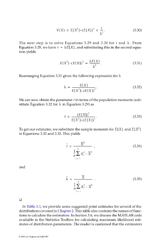
The next step is to solve Equations 3.29 and 3.30 for t and . From
Equation 3.29, we have t = λEX[] , and substituting this in the second equa-
tion yields
[
2
2
----------------
EX ] ( – EX[]) = λEX[] . (3.31)
λ 2
Rearranging Equation 3.31 gives the following expression for λ
EX[]
λ = --------------------------------------- . (3.32)
[
2
EX ] ( – EX[]) 2
We can now obtain the parameter t in terms of the population moments (sub-
λ
stitute Equation 3.32 for in Equation 3.29) as
( EX[]) 2
t = --------------------------------------- . (3.33)
2
[
EX ] ( – EX[]) 2
2
[
To get our estimates, we substitute the sample moments for EX[] and EX ]
in Equations 3.32 and 3.33. This yields
2
ˆ X
t = ------------------------------ , (3.34)
n
1 2
--- ∑ X i – X
2
n
i = 1
and

ˆ X
λ = ------------------------------ . (3.35)
n
1 2
--- ∑ X i – X
2
n
i = 1

In Table 3.1, we provide some suggested point estimates for several of the
distributions covered in Chapter 2. This table also contains the names of func-
tions to calculate the estimators. In Section 3.6, we discuss the MATLAB code
available in the Statistics Toolbox for calculating maximum likelihood esti-
mates of distribution parameters. The reader is cautioned that the estimators

© 2002 by Chapman & Hall/CRC