Page 79 - Computational Statistics Handbook with MATLAB

Chapter 3: Sampling Concepts 65

n
1
2
--- ln
--- ln
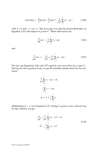
ln [ L θ()] = – n [ 2π] – n [ σ ] – --------- 2∑ ( x – µ) 2 , (3.25)
i
2 2 2σ
i = 1
with σ > 0 and ∞ <– µ < ∞ . The next step is to take the partial derivative of
Equation 3.25 with respect to µ and σ 2 . These derivatives are
n
∂ 1 ( µ)
∂ µ ln L = ----- 2∑ x i – , (3.26)
σ
i = 1
and

n
∂ n 1 2
ln L = – --------- + --------- 4∑ ( x i – µ) . (3.27)
∂ σ 2 2σ 2 2σ
i = 1
We then set Equations 3.26 and 3.27 equal to zero and solve for µ and σ 2 .
Solving the first equation for µ, we get the familiar sample mean for the esti-
mator.

n
1
----- 2∑ ( x i – µ) = 0,
σ
i = 1
n
∑ x i = nµ,

i = 1
n
ˆ 1
µ = x = --- ∑ x i .
n
i = 1
ˆ
Substituting µ = x into Equation 3.27, setting it equal to zero, and solving
for the variance, we get

n
n 1 2
– --------- + --------- 4∑ ( x i – x) = 0
2σ 2 2σ
i = 1
(3.28)
n
ˆ 2 1 2
σ = --- ∑ ( x i – x) .
n
i = 1

© 2002 by Chapman & Hall/CRC