Page 202 -

Section 6.1 Local Texture Representations Using Filters 170

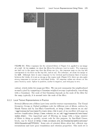
FIGURE 6.6: Filter responses for the oriented filters of Figure 6.4, applied to an image
of a wall. At the center, we show the filters for reference (not to scale). The responses
are laid out in the same way that the filters are (i.e., the response map on the top left
corresponds to the filter on the top left, and so on). For reference, we show the image at
the left. Although there is some response to the vertical and horizontal lines of mortar
between the bricks, it is not as strong as the coarse scale (Figure 6.5); there are also quite
strong responses to texture on individual bricks. All response values are shown on the
same intensity scale: lighter is positive, darker is negative, and mid-gray is zero.

cation), which yields two maps per filter. We can now summarize the neighborhood
around a pixel by computing a Gaussian weighted average (equivalently, convolving
with a Gaussian). The scale of this Gaussian depends on the scale of the filter for
the map; typically, it is around twice the scale of the filter.

6.1.3 Local Texture Representations in Practice
Several different sets of filters have been used for texture representation. The Visual
Geometry Group at Oxford publishes code for different sets of filters, written by
Manik Varma and by Jan-Mark Guesebroek, at http://www.robots.ox.ac.uk/
~ vgg/research/texclass/filters.html; this is part of an excellent web page on
texture classification (http://www.robots.ox.ac.uk/ ~ vgg/research/texclass/
index.html). One important part of filtering an image with a large number
of filters is doing so quickly; recent code for this purpose, by Jan-Mark Guese-
broek, can be found at http://www.science.uva.nl/research/publications/
2003/GeusebroekTIP2003/. Some sets of oriented filters allow fast, efficient rep-
resentations and have good translation and rotation properties. One such set is