Page 425 -

Section 13.1 Elements of Differential Geometry 393

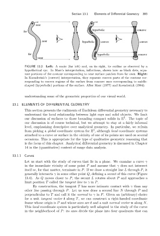
FIGURE 13.2: Left: A snake (far left) and, on its right, its outline as observed by a
hypothetical eye. In Marr’s interpretation, inflections, shown here as black dots, sepa-
rate portions of the contour corresponding to near surface patches from far ones. Right:
In Koenderink’s (correct) interpretation, they separate convex parts of the contour cor-
responding to convex regions of the surface from concave ones corresponding to saddle-
shaped (hyperbolic) portions of the surface. After Marr (1977) and Koenderink (1984).

understanding some of the geometric properties of our visual world.

13.1 ELEMENTS OF DIFFERENTIAL GEOMETRY
This section presents the rudiments of Euclidean differential geometry necessary to
understand the local relationship between light rays and solid objects. We limit
3
our discussion of surfaces to those bounding compact solids in E . The topic of
our discussion is of course technical, but we attempt to stay at a fairly informal
level, emphasizing descriptive over analytical geometry. In particular, we refrain
3
from picking a global coordinate system for E , although local coordinate systems
attached to a curve or surface in the vicinity of one of its points are used on several
occasions. This is appropriate for the type of qualitative geometric reasoning that
is the focus of this chapter. Analytical differential geometry is discussed in Chapter
14 in the (quantitative) context of range data analysis.

13.1.1 Curves
Let us start with the study of curves that lie in a plane. We examine a curve γ
in the immediate vicinity of some point P and assume that γ does not intersect
itself or, for that matter, terminate in P. If we draw a straight line L through P,it
generally intersects γ in some other point Q, defining a secant of this curve (Figure
13.4). As Q moves closer to P, the secant L rotates about P and approaches a
limit position T called the tangent line to γ in P.
By construction, the tangent T has more intimate contact with γ than any
other line passing through P. Let us now draw a second line N through P and
perpendicular to T and call it the normal to γ in P. Given an (arbitrary) choice
for a unit tangent vector t along T , we can construct a right-handed coordinate
frame whose origin is P and whose axes are t and a unit normal vector n along N.
This local coordinate system is particularly well adapted to the study of the curve
in the neighborhood of P: its axes divide the plane into four quadrants that can