Page 56 -

2.1 Geometric primitives and transformations 35

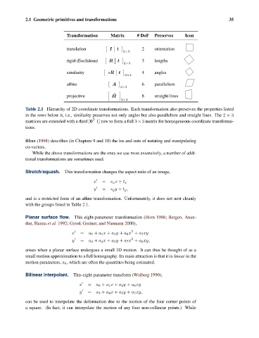
Transformation Matrix # DoF Preserves Icon

translation I t 2 orientation
2×3

rigid (Euclidean) R t 3 lengths
2×3

similarity sR t 4 angles
2×3

affine A 6 parallelism
2×3

˜

projective H 8 straight lines
3×3
Table 2.1 Hierarchy of 2D coordinate transformations. Each transformation also preserves the properties listed
in the rows below it, i.e., similarity preserves not only angles but also parallelism and straight lines. The 2 × 3
T
matrices are extended with a third [0 1] row to form a full 3 × 3 matrix for homogeneous coordinate transforma-
tions.
Blinn (1998) describes (in Chapters 9 and 10) the ins and outs of notating and manipulating
co-vectors.
While the above transformations are the ones we use most extensively, a number of addi-
tional transformations are sometimes used.

Stretch/squash. This transformation changes the aspect ratio of an image,

x = s x x + t x
y = s y y + t y ,
and is a restricted form of an affine transformation. Unfortunately, it does not nest cleanly
with the groups listed in Table 2.1.

Planar surface flow. This eight-parameter transformation (Horn 1986; Bergen, Anan-
dan, Hanna et al. 1992; Girod, Greiner, and Niemann 2000),
2
x = a 0 + a 1 x + a 2 y + a 6 x + a 7 xy
2
y = a 3 + a 4 x + a 5 y + a 7 x + a 6 xy,
arises when a planar surface undergoes a small 3D motion. It can thus be thought of as a
small motion approximation to a full homography. Its main attraction is that it is linear in the
motion parameters, a k , which are often the quantities being estimated.

Bilinear interpolant. This eight-parameter transform (Wolberg 1990),
x = a 0 + a 1 x + a 2 y + a 6 xy
y = a 3 + a 4 x + a 5 y + a 7 xy,

can be used to interpolate the deformation due to the motion of the four corner points of
a square. (In fact, it can interpolate the motion of any four non-collinear points.) While