Page 51 -

30 2 Image formation

z ^
y n n
^
l
m
d
ș x d
x y
(a) (b)

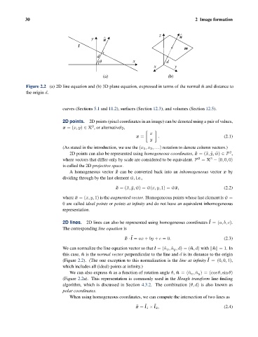
Figure 2.2 (a) 2D line equation and (b) 3D plane equation, expressed in terms of the normal ˆn and distance to
the origin d.

curves (Sections 5.1 and 11.2), surfaces (Section 12.3), and volumes (Section 12.5).

2D points. 2D points (pixel coordinates in an image) can be denoted using a pair of values,
2
x =(x, y) ∈R , or alternatively,

x
x = . (2.1)
y
(As stated in the introduction, we use the (x 1 ,x 2 ,...) notation to denote column vectors.)
2
2D points can also be represented using homogeneous coordinates, ˜x =(˜x, ˜y, ˜w) ∈P ,
2
3
where vectors that differ only by scale are considered to be equivalent. P = R − (0, 0, 0)
is called the 2D projective space.
A homogeneous vector ˜x can be converted back into an inhomogeneous vector x by
dividing through by the last element ˜w, i.e.,

˜ x =(˜x, ˜y, ˜w)= ˜w(x, y, 1) = ˜w¯x, (2.2)
where ¯x =(x, y, 1) is the augmented vector. Homogeneous points whose last element is ˜w =
0 are called ideal points or points at infinity and do not have an equivalent inhomogeneous
representation.

˜
2D lines. 2D lines can also be represented using homogeneous coordinates l =(a, b, c).
The corresponding line equation is
˜
¯ x · l = ax + by + c =0. (2.3)
We can normalize the line equation vector so that l =(ˆn x , ˆn y ,d)=(ˆn,d) with ˆn =1.In
this case, ˆn is the normal vector perpendicular to the line and d is its distance to the origin
˜
(Figure 2.2). (The one exception to this normalization is the line at infinity l =(0, 0, 1),
which includes all (ideal) points at infinity.)
We can also express ˆn as a function of rotation angle θ, ˆn =(ˆn x , ˆn y ) = (cos θ, sin θ)
(Figure 2.2a). This representation is commonly used in the Hough transform line-finding
algorithm, which is discussed in Section 4.3.2. The combination (θ, d) is also known as
polar coordinates.
When using homogeneous coordinates, we can compute the intersection of two lines as
˜ ˜
˜ x = l 1 × l 2 , (2.4)