Page 53 -

32 2 Image formation

z
p
Ȝ
r=(1-Ȝ)p+Ȝq

q
x y

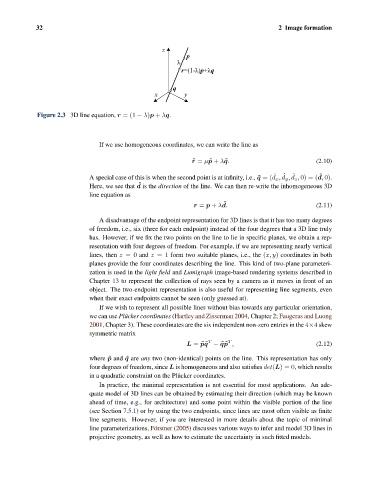
Figure 2.3 3D line equation, r =(1 − λ)p + λq.

If we use homogeneous coordinates, we can write the line as

˜ r = μ˜p + λ˜q. (2.10)

ˆ
ˆ ˆ ˆ
A special case of this is when the second point is at infinity, i.e., ˜q =(d x , d y , d z , 0)=(d, 0).
ˆ
Here, we see that d is the direction of the line. We can then re-write the inhomogeneous 3D
line equation as
ˆ
r = p + λd. (2.11)
A disadvantage of the endpoint representation for 3D lines is that it has too many degrees
of freedom, i.e., six (three for each endpoint) instead of the four degrees that a 3D line truly
has. However, if we fix the two points on the line to lie in specific planes, we obtain a rep-
resentation with four degrees of freedom. For example, if we are representing nearly vertical
lines, then z =0 and z =1 form two suitable planes, i.e., the (x, y) coordinates in both
planes provide the four coordinates describing the line. This kind of two-plane parameteri-
zation is used in the light field and Lumigraph image-based rendering systems described in
Chapter 13 to represent the collection of rays seen by a camera as it moves in front of an
object. The two-endpoint representation is also useful for representing line segments, even
when their exact endpoints cannot be seen (only guessed at).
If we wish to represent all possible lines without bias towards any particular orientation,
we can use Pl¨ ucker coordinates (Hartley and Zisserman 2004, Chapter 2; Faugeras and Luong
2001, Chapter 3). These coordinates are the six independent non-zero entries in the 4×4 skew
symmetric matrix
T
T
L = ˜p˜q − ˜q˜p , (2.12)
where ˜p and ˜q are any two (non-identical) points on the line. This representation has only
four degrees of freedom, since L is homogeneous and also satisfies det(L)=0, which results
in a quadratic constraint on the Pl¨ ucker coordinates.
In practice, the minimal representation is not essential for most applications. An ade-
quate model of 3D lines can be obtained by estimating their direction (which may be known
ahead of time, e.g., for architecture) and some point within the visible portion of the line
(see Section 7.5.1) or by using the two endpoints, since lines are most often visible as finite
line segments. However, if you are interested in more details about the topic of minimal
line parameterizations, F¨ orstner (2005) discusses various ways to infer and model 3D lines in
projective geometry, as well as how to estimate the uncertainty in such fitted models.