Page 62 -

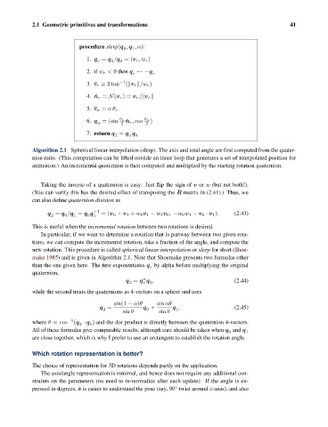
2.1 Geometric primitives and transformations 41

procedure slerp(q , q ,α):
0
1
1. q = q /q =(v r ,w r )
1
r
0
2. if w r < 0 then q ←−q r
r
3. θ r = 2 tan −1 ( v r /w r )
4. ˆn r = N(v r )= v r / v r

5. θ α = αà r
6. q = (sin θ α ˆ n r , cos θ α )
α 2 2
7. return q = q q
2
α 0
Algorithm 2.1 Spherical linear interpolation (slerp). The axis and total angle are first computed from the quater-
nion ratio. (This computation can be lifted outside an inner loop that generates a set of interpolated position for
animation.) An incremental quaternion is then computed and multiplied by the starting rotation quaternion.

Taking the inverse of a quaternion is easy: Just flip the sign of v or w (but not both!).
(You can verify this has the desired effect of transposing the R matrix in (2.41).) Thus, we
can also define quaternion division as

q = q /q = q q −1 =(v 0 × v 1 + w 0 v 1 − w 1 v 0 , −w 0 w 1 − v 0 · v 1 ). (2.43)
0 1
1
2
0
This is useful when the incremental rotation between two rotations is desired.
In particular, if we want to determine a rotation that is partway between two given rota-
tions, we can compute the incremental rotation, take a fraction of the angle, and compute the
new rotation. This procedure is called spherical linear interpolation or slerp for short (Shoe-
make 1985) and is given in Algorithm 2.1. Note that Shoemake presents two formulas other
than the one given here. The first exponentiates q by alpha before multiplying the original
r
quaternion,
α
q = q q , (2.44)
2
r
0
while the second treats the quaternions as 4-vectors on a sphere and uses
sin(1 − α)θ sin αà
q = q + q , (2.45)
2 0 1
sin θ sin θ
where θ =cos −1 (q · q ) and the dot product is directly between the quaternion 4-vectors.
0
1
All of these formulas give comparable results, although care should be taken when q and q 1
0
are close together, which is why I prefer to use an arctangent to establish the rotation angle.
Which rotation representation is better?
The choice of representation for 3D rotations depends partly on the application.
The axis/angle representation is minimal, and hence does not require any additional con-
straints on the parameters (no need to re-normalize after each update). If the angle is ex-
◦
pressed in degrees, it is easier to understand the pose (say, 90 twist around x-axis), and also