Page 65 -

44 2 Image formation

orientation) can be estimated using simple least squares (Section 6.2.1). Under orthography,
structure and motion can simultaneously be estimated using factorization (singular value de-
composition), as discussed in Section 7.3 (Tomasi and Kanade 1992).
A closely related projection model is para-perspective (Aloimonos 1990; Poelman and
Kanade 1997). In this model, object points are again first projected onto a local reference
parallel to the image plane. However, rather than being projected orthogonally to this plane,
they are projected parallel to the line of sight to the object center (Figure 2.7d). This is
followed by the usual projection onto the final image plane, which again amounts to a scaling.
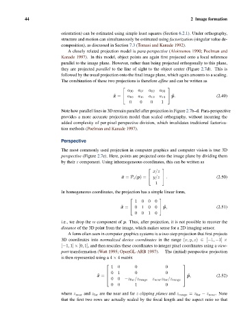
The combination of these two projections is therefore affine and can be written as

⎡ ⎤
a 00 a 01 a 02 a 03
˜ x = ⎣ a 10 a 11 a 12 a 13 ⎦ ˜ p. (2.49)
0 0 0 1

Note how parallel lines in 3D remain parallel after projection in Figure 2.7b–d. Para-perspective
provides a more accurate projection model than scaled orthography, without incurring the
added complexity of per-pixel perspective division, which invalidates traditional factoriza-
tion methods (Poelman and Kanade 1997).

Perspective
The most commonly used projection in computer graphics and computer vision is true 3D
perspective (Figure 2.7e). Here, points are projected onto the image plane by dividing them
by their z component. Using inhomogeneous coordinates, this can be written as
x/z
⎡ ⎤
¯ x = P z (p)= ⎣ y/z ⎦ . (2.50)
1

In homogeneous coordinates, the projection has a simple linear form,

1000
⎡ ⎤
˜ x = ⎣ 0100 ⎦ ˜ p, (2.51)
0010
i.e., we drop the w component of p. Thus, after projection, it is not possible to recover the
distance of the 3D point from the image, which makes sense for a 2D imaging sensor.
A form often seen in computer graphics systems is a two-step projection that first projects
3D coordinates into normalized device coordinates in the range (x, y, z) ∈ [−1, −1] ×
[−1, 1] × [0, 1], and then rescales these coordinates to integer pixel coordinates using a view-
port transformation (Watt 1995; OpenGL-ARB 1997). The (initial) perspective projection
is then represented using a 4 × 4 matrix

10 0 0
⎡ ⎤
01 0 0
⎢ ⎥
˜ x = ⎢ ⎥ ˜ p, (2.52)
⎣ 00 −z far /z range z near z far /z range ⎦
00 1 0
where z near and z far are the near and far z clipping planes and z range = z far − z near . Note
that the first two rows are actually scaled by the focal length and the aspect ratio so that