Page 68 -

2.1 Geometric primitives and transformations 47

W-1
y c
0 x s

0 (c x,c y) f
z c
x c
H-1
y s

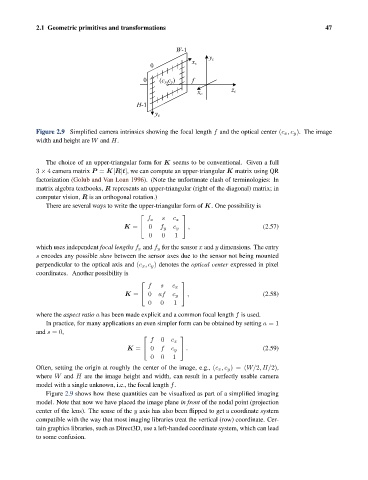
Figure 2.9 Simplified camera intrinsics showing the focal length f and the optical center (c x ,c y ). The image
width and height are W and H.

The choice of an upper-triangular form for K seems to be conventional. Given a full
3 × 4 camera matrix P = K[R|t], we can compute an upper-triangular K matrix using QR
factorization (Golub and Van Loan 1996). (Note the unfortunate clash of terminologies: In
matrix algebra textbooks, R represents an upper-triangular (right of the diagonal) matrix; in
computer vision, R is an orthogonal rotation.)
There are several ways to write the upper-triangular form of K. One possibility is
⎡ ⎤
f x s c x
K = ⎣ 0 f y c y ⎦ , (2.57)
0 0 1

which uses independent focal lengths f x and f y for the sensor x and y dimensions. The entry
s encodes any possible skew between the sensor axes due to the sensor not being mounted
perpendicular to the optical axis and (c x ,c y ) denotes the optical center expressed in pixel
coordinates. Another possibility is
f s c x
⎡ ⎤
K = ⎣ 0 af c y ⎦ , (2.58)
0 0 1

where the aspect ratio a has been made explicit and a common focal length f is used.
In practice, for many applications an even simpler form can be obtained by setting a =1
and s =0,
f 0 c x
⎡ ⎤
K = ⎣ 0 f c y ⎦ . (2.59)
0 0 1
Often, setting the origin at roughly the center of the image, e.g., (c x ,c y )=(W/2,H/2),
where W and H are the image height and width, can result in a perfectly usable camera
model with a single unknown, i.e., the focal length f.
Figure 2.9 shows how these quantities can be visualized as part of a simplified imaging
model. Note that now we have placed the image plane in front of the nodal point (projection
center of the lens). The sense of the y axis has also been flipped to get a coordinate system
compatible with the way that most imaging libraries treat the vertical (row) coordinate. Cer-
tain graphics libraries, such as Direct3D, use a left-handed coordinate system, which can lead
to some confusion.