Page 71 -

50 2 Image formation

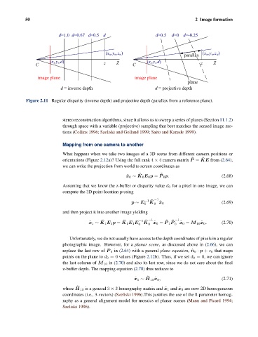
d=1.0 d=0.67 d=0.5 d d=0.5 d=0 d=-0.25

(x w,y w,z w) parallax (x w,y w,z w)
(x s,y s,d) z Z (x s,y s,d) z Z
C C

image plane image plane
plane
d = inverse depth d = projective depth

Figure 2.11 Regular disparity (inverse depth) and projective depth (parallax from a reference plane).

stereo reconstruction algorithms, since it allows us to sweep a series of planes (Section 11.1.2)
through space with a variable (projective) sampling that best matches the sensed image mo-
tions (Collins 1996; Szeliski and Golland 1999; Saito and Kanade 1999).

Mapping from one camera to another

What happens when we take two images of a 3D scene from different camera positions or
˜ ˜
orientations (Figure 2.12a)? Using the full rank 4 × 4 camera matrix P = KE from (2.64),
we can write the projection from world to screen coordinates as
˜
˜
˜ x 0 ∼ K 0 E 0 p = P 0 p. (2.68)
Assuming that we know the z-buffer or disparity value d 0 for a pixel in one image, we can
compute the 3D point location p using
−1 ˜ −1
p ∼ E K (2.69)
0 0 ˜ x 0
and then project it into another image yielding
˜
˜
˜ ˜
K
˜ x 1 ∼ K 1 E 1 p = K 1 E 1 E −1 ˜ −1 ˜ x 0 = P 1 P −1 ˜ x 0 = M 10 ˜ x 0 . (2.70)
0 0 0
Unfortunately, we do not usually have access to the depth coordinates of pixels in a regular
photographic image. However, for a planar scene, as discussed above in (2.66), we can
replace the last row of P 0 in (2.64) with a general plane equation, ˆn 0 · p + c 0 that maps
points on the plane to d 0 =0 values (Figure 2.12b). Thus, if we set d 0 =0, we can ignore
the last column of M 10 in (2.70) and also its last row, since we do not care about the final
z-buffer depth. The mapping equation (2.70) thus reduces to
˜
˜ x 1 ∼ H 10 ˜ x 0 , (2.71)
˜
where H 10 is a general 3 × 3 homography matrix and ˜ x 1 and ˜ x 0 are now 2D homogeneous
coordinates (i.e., 3-vectors) (Szeliski 1996).This justifies the use of the 8-parameter homog-
raphy as a general alignment model for mosaics of planar scenes (Mann and Picard 1994;
Szeliski 1996).