Page 66 -

2.1 Geometric primitives and transformations 45

y c
x s
s x
p c
c s
s y
O c z c
p x c
y s

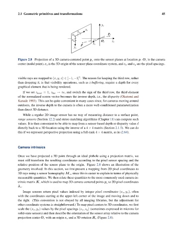
Figure 2.8 Projection of a 3D camera-centered point p onto the sensor planes at location p. O c is the camera
c
center (nodal point), c s is the 3D origin of the sensor plane coordinate system, and s x and s y are the pixel spacings.

2
visible rays are mapped to (x, y, z) ∈ [−1, −1] . The reason for keeping the third row, rather
than dropping it, is that visibility operations, such as z-buffering, require a depth for every
graphical element that is being rendered.
If we set z near =1, z far →∞, and switch the sign of the third row, the third element
of the normalized screen vector becomes the inverse depth, i.e., the disparity (Okutomi and
Kanade 1993). This can be quite convenient in many cases since, for cameras moving around
outdoors, the inverse depth to the camera is often a more well-conditioned parameterization
than direct 3D distance.
While a regular 2D image sensor has no way of measuring distance to a surface point,
range sensors (Section 12.2) and stereo matching algorithms (Chapter 11) can compute such
values. It is then convenient to be able to map from a sensor-based depth or disparity value d
directly back to a 3D location using the inverse of a 4 × 4 matrix (Section 2.1.5). We can do
this if we represent perspective projection using a full-rank 4 × 4 matrix, as in (2.64).

Camera intrinsics

Once we have projected a 3D point through an ideal pinhole using a projection matrix, we
must still transform the resulting coordinates according to the pixel sensor spacing and the
relative position of the sensor plane to the origin. Figure 2.8 shows an illustration of the
geometry involved. In this section, we first present a mapping from 2D pixel coordinates to
3D rays using a sensor homography M s , since this is easier to explain in terms of physically
measurable quantities. We then relate these quantities to the more commonly used camera in-
trinsic matrix K, which is used to map 3D camera-centered points p to 2D pixel coordinates
c
˜ x s .
Image sensors return pixel values indexed by integer pixel coordinates (x s ,y s ), often
with the coordinates starting at the upper-left corner of the image and moving down and to
the right. (This convention is not obeyed by all imaging libraries, but the adjustment for
other coordinate systems is straightforward.) To map pixel centers to 3D coordinates, we first
scale the (x s ,y s ) values by the pixel spacings (s x ,s y ) (sometimes expressed in microns for
solid-state sensors) and then describe the orientation of the sensor array relative to the camera
projection center O c with an origin c s and a 3D rotation R s (Figure 2.8).