Page 85 - Control Theory in Biomedical Engineering

72 Control theory in biomedical engineering

n P n P n P n P
z ,v ∗ fg fg fg
∗
k
i i i¼0 :¼ arg min J n P ,k γ , q i i¼0 , v i i¼0 , z i i¼0
v U, z Z
z i +1 ¼ A k z i + B k v i + d i , 8i 
8 n P 1
> 0 (4)
<
s:t: q i ¼ C k z i , 8i  n P
0
>
:
z 0 ¼ x k
with the objective function
n P
X
T
n P n P
ð
fg
fg
k
J n P ,k q i ,γ , v i i¼0 , z i i¼0 :¼ ð q i r k,i Þ Q k q i r k,i Þ
i¼0
T
+ v i I db;i R k v i I db;i
+ e PIC P k e PIC
i i
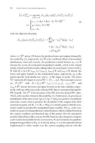
where z i  and q i  denote the predicted states and outputs obtained by
n x
the model Eq. (2), respectively, d i  is the combined effects of unmodeled
disturbances, meal and exercise, the prediction/control horizon n P , v i 
denotes the vector of constrained manipulated variable, which is the infused
insulin as basal and bolus insulin, taking values in a nonempty convex set U
 with U :¼ ν  : ν min ν ν max g, ν min  and ν max  denote the
f
lower and upper bounds on the manipulated input, respectively, I db is the
patient-specific basal insulin rate, and r k, i is the target set-point. The index
 represents all integers in a set as  :¼ 0,…,n P g. The nonempty convex
n P
n P
f
0 0

set Z  n x with Z :¼ z  : z min z z max , z min  n x and
n x
z max  denote the lower and upper bounds on the state variables, respec-
n x
tively,withoneofthestatesastheestimatedPICthatisconstrainedthroughthe
PIC bounds. The e PIC is the deviation of the PIC from the desired PIC value.
i
Then x isthenumberofstatesinthemodelEq.(2).Furthermore,x k providesan
initialization of the state vector, Q k 0, Q k :¼ Q yðÞ is a positive semidefinite
k
symmetric matrix used to penalize the deviations of the outputs from their
nominal set-point, and R k > 0, R k :¼ R γðÞ is a strictly positive definite sym-
k
metric matrix to penalize the manipulated input variables. The r k, i is the con-
trollerset-pointovertheprediction/controlhorizon,whichisdefinedbasedon
the current condition and historical data of the patient. For the anticipated
periodsofdisturbanceslikeexercise,thePIClimitsarealsochangedtocompute
asaferinsulindosesuitablefortheexercisetime.Ateachiteration,thequadratic
programming problem in Eq. (4)is solved, and u k :¼ v 0 is the optimal solution
implemented to infuse insulin over the current sampling interval with the