Page 142 - Corrosion Engineering Principles and Practice

116 C h a p t e r 5 C o r r o s i o n K i n e t i c s a n d A p p l i c a t i o n s o f E l e c t r o c h e m i s t r y 117

where R is the solution resistance
s
R is the polarization resistance
p
w is the frequency
C is the double layer capacitance
dl
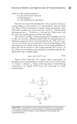
The term Q, in Fig. 5.25, describes the “leaky capacitor” behavior
corresponding to the presence of a constant-phase element (CPE)
[12]. Figure 5.26(a) illustrates the complex plane presentation of the
EIS model circuit in Fig. 5.25(a) where R = 10 Ω, R = 100 kΩ and Q
p
s
decomposes into C = 40 µF and n = 0.8 and Fig. 5.26(b) shows how
dl
the same data would appear in a Bode plot format.
The second circuit [Fig. 5.25(b)] was proposed by Hladky et al. [13].
to take into account a diffusion-limited behavior corresponding to a
Warburg component which can be described by Eq. (5.26). The expo-
nent n in Eq. (5.26) can vary between 0.5 and 0.25 depending on the
smoothness of the metallic surface that is 0.5 for highly polished sur-
faces and 0.25 for porous or very rough materials [14]. R and C in
Eq. (5.26), are the resistance and capacitance associated with the dis-
tributed R-C line of infinite length.
Z( ) = (0.5 i R C) 0.5 i w − n (5.26)
w
/
Figure 5.27(a) illustrates the complex plane presentation of
simulated data corresponding to model circuit in Fig. 5.25(b) where
R = 10 Ω, R = 100 kΩ, C = 40 µF, and the exponent n of the Warburg
p
dl
s
component = 0.4. Figure 5.27(b) shows the same data in a Bode
representation.

R p
R s
Q

(a)
C dl
R s

W
R p
(b)
FIGURE 5.25 The equivalent circuit models proposed for the interpretation
of EIS results measured in corroding systems: (a) simplest representation
of an electrochemical interface, (b) one relaxation time constant with
extended diffusion.