Page 138 - Corrosion Engineering Principles and Practice

112 C h a p t e r 5 C o r r o s i o n K i n e t i c s a n d A p p l i c a t i o n s o f E l e c t r o c h e m i s t r y 113

The Tafel slopes in this equation can be evaluated experimentally
using real polarization plots in the fashion described in Fig. 5.3 or
obtained from the literature [8]. The corrosion currents may then be
converted into other corrosion rate units using Faraday’s law or, more
simply, by using a conversion scheme provided in Chap. 3, that is,
Table 3.1 for all metals, or Table 3.2 adapted to iron or steel.
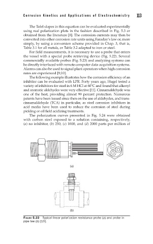
For field measurements, it is necessary to use a probe that enters
the vessel with a special probe retrieving device (Fig. 5.22). Several
commercially available probes (Fig. 5.23) and analyzing systems can
be directly interfaced with remote computer data-acquisition systems.
Alarms can also be used to signal plant operators when high corrosion
rates are experienced [9;10].
The following example illustrates how the corrosion efficiency of an
inhibitor can be evaluated with LPR. Forty years ago, Hugel tested a
variety of inhibitors for steel in 6 M HCl at 60°C and found that alkenyl
and aromatic aldehydes were very effective [11]. Cinnamaldehyde was
one of the best, providing almost 99 percent protection. Numerous
patents have been issued since then on the use of aldehydes, and trans-
cinnamaldehyde (TCA) in particular, as steel corrosion inhibitors in
acid media have been used to reduce the corrosion of steel during
pickling or oil field acidizing treatments.
The polarization curves presented in Fig. 5.24 were obtained
with carbon steel exposed to a solution containing, respectively,
(a) no inhibitor, (b) 250, (c) 1000, and (d) 2000 parts per million of

(a)

(b)

FIGURE 5.22 Typical linear polarization resistance probe (a) and probe in
pipe tee (b) [10].