Page 137 - Corrosion Engineering Principles and Practice

112 C h a p t e r 5 C o r r o s i o n K i n e t i c s a n d A p p l i c a t i o n s o f E l e c t r o c h e m i s t r y 113

Coupon immersion tests confirmed the long-term predictions.
Slight attack was found under the artificial crevice formers in the
complete liquid exposure. The practical conclusion of this in-service
study was that, since localized corrosion often takes time to develop,
a few days of exposure to this chemical product could be acceptable.
However, it was recommended to avoid long-term exposure since
both pitting and crevice corrosion would be expected for longer
exposure periods.

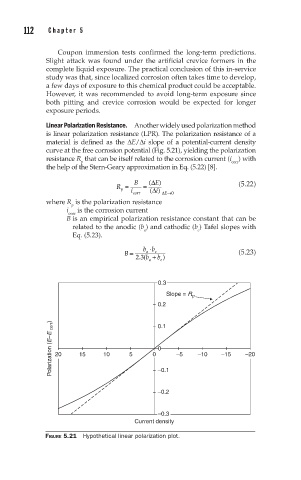
Linear Polarization Resistance. Another widely used polarization method
is linear polarization resistance (LPR). The polarization resistance of a
material is defined as the ∆E/∆i slope of a potential-current density
curve at the free corrosion potential (Fig. 5.21), yielding the polarization
resistance R that can be itself related to the corrosion current (i ) with
p
corr
the help of the Stern-Geary approximation in Eq. (5.22) [8].
R = B = (∆ E) (5.22)
p i corr (∆ i) ∆ E→0
where R is the polarization resistance
p
i corr is the corrosion current
B is an empirical polarization resistance constant that can be
related to the anodic (b ) and cathodic (b ) Tafel slopes with
a
c
Eq. (5.23).
⋅
B = b b c (5.23)
a
2 3. ( b + b )
c
a
0.3
Slope = R p
0.2

Polarization (E–E corr ) 20 15 10 5 0 0 –5 –10 –15 –20
0.1

–0.1

–0.2

–0.3
Current density
FIGURE 5.21 Hypothetical linear polarization plot.