Page 390 - Corrosion Engineering Principles and Practice

358 C h a p t e r 9 A t m o s p h e r i c C o r r o s i o n 359

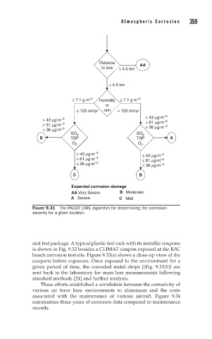
Distance AA
to sea ≤ 4.5 km

> 4.5 km

≤ 7.1 g m –3 Humidity ≤ 7.1 g m –3
or
≤ 125 cm/yr rain > 125 cm/yr
–3
> 43 mg m –3 > 43 mg m
–3
> 61 mg m
–3
> 61 mg m > 36 mg m –3
> 36 mg m –3
SO SO
2
2
B TSP TSP A
O 3 O 3
≤ 43 mg m –3 ≤ 43 mg m –3
≤ 61 mg m –3 ≤ 61 mg m –3
≤ 36 mg m –3 ≤ 36 mg m –3
C B
Expected corrosion damage
AA Very Severe B Moderate
A Severe C Mild

FIGURE 9.31 The PACER LIME algorithm for determining the corrosion
severity for a given location.

and test package. A typical plastic test rack with its metallic coupons
is shown in Fig. 9.32 besides a CLIMAT coupon exposed at the KSC
beach corrosion test site. Figure 9.33(a) shows a close-up view of the
coupons before exposure. Once exposed to the environment for a
given period of time, the corroded metal strips [(Fig. 9.33(b)] are
sent back to the laboratory for mass loss measurements following
standard methods [24] and further analysis.
These efforts established a correlation between the corrosivity of
various air force base environments to aluminum and the costs
associated with the maintenance of various aircraft. Figure 9.34
summarizes three years of corrosion data compared to maintenance
records.