Page 133 -

HAN 10-ch03-083-124-9780123814791

96 Chapter 3 Data Preprocessing 2011/6/1 3:16 Page 96 #14

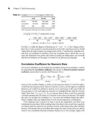
Table 3.1 Example 2.1’s 2 × 2 Contingency Table Data
male female Total
fiction 250 (90) 200 (360) 450
non fiction 50 (210) 1000 (840) 1050
Total 300 1200 1500
Note: Are gender and preferred reading correlated?
2
Using Eq. (3.1) for χ computation, we get

(250 − 90) 2 (50 − 210) 2 (200 − 360) 2 (1000 − 840) 2
2
χ = + + +
90 210 360 840
= 284.44 + 121.90 + 71.11 + 30.48 = 507.93.
For this 2 × 2 table, the degrees of freedom are (2 − 1)(2 − 1) = 1. For 1 degree of free-
2
dom, the χ value needed to reject the hypothesis at the 0.001 significance level is 10.828
2
(taken from the table of upper percentage points of the χ distribution, typically avail-
able from any textbook on statistics). Since our computed value is above this, we can
reject the hypothesis that gender and preferred reading are independent and conclude
that the two attributes are (strongly) correlated for the given group of people.

Correlation Coefficient for Numeric Data
For numeric attributes, we can evaluate the correlation between two attributes, A and B,
by computing the correlation coefficient (also known as Pearson’s product moment
coefficient, named after its inventer, Karl Pearson). This is
n n
X X
¯
¯
(a i − A)(b i − ¯ B) (a i b i ) − nA ¯ B
i=1 i=1
r A,B = = , (3.3)
nσ A σ B nσ A σ B
where n is the number of tuples, a i and b i are the respective values of A and B in tuple i,
¯
A and ¯ B are the respective mean values of A and B, σ A and σ B are the respective standard
deviations of A and B (as defined in Section 2.2.2), and 6(a i b i ) is the sum of the AB
cross-product (i.e., for each tuple, the value for A is multiplied by the value for B in that
tuple). Note that −1 ≤ r A,B ≤ +1. If r A,B is greater than 0, then A and B are positively
correlated, meaning that the values of A increase as the values of B increase. The higher
the value, the stronger the correlation (i.e., the more each attribute implies the other).
Hence, a higher value may indicate that A (or B) may be removed as a redundancy.
If the resulting value is equal to 0, then A and B are independent and there is no
correlation between them. If the resulting value is less than 0, then A and B are negatively
correlated, where the values of one attribute increase as the values of the other attribute
decrease. This means that each attribute discourages the other. Scatter plots can also be
used to view correlations between attributes (Section 2.2.3). For example, Figure 2.8’s