Page 138 -

10-ch03-083-124-9780123814791
2011/6/1
3:16 Page 101
HAN
#19
3.4 Data Reduction 101

cleaning as well. Given a set of coefficients, an approximation of the original data can be
constructed by applying the inverse of the DWT used.
The DWT is closely related to the discrete Fourier transform (DFT), a signal process-
ing technique involving sines and cosines. In general, however, the DWT achieves better
lossy compression. That is, if the same number of coefficients is retained for a DWT and
a DFT of a given data vector, the DWT version will provide a more accurate approxima-
tion of the original data. Hence, for an equivalent approximation, the DWT requires less
space than the DFT. Unlike the DFT, wavelets are quite localized in space, contributing
to the conservation of local detail.
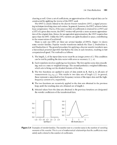
There is only one DFT, yet there are several families of DWTs. Figure 3.4 shows
some wavelet families. Popular wavelet transforms include the Haar-2, Daubechies-4,
and Daubechies-6. The general procedure for applying a discrete wavelet transform uses
a hierarchical pyramid algorithm that halves the data at each iteration, resulting in fast
computational speed. The method is as follows:
1. The length, L, of the input data vector must be an integer power of 2. This condition
can be met by padding the data vector with zeros as necessary (L ≥ n).
2. Each transform involves applying two functions. The first applies some data smooth-
ing, such as a sum or weighted average. The second performs a weighted difference,
which acts to bring out the detailed features of the data.
3. The two functions are applied to pairs of data points in X, that is, to all pairs of
measurements (x 2i ,x 2i+1 ). This results in two data sets of length L/2. In general,
these represent a smoothed or low-frequency version of the input data and the high-
frequency content of it, respectively.
4. The two functions are recursively applied to the data sets obtained in the previous
loop, until the resulting data sets obtained are of length 2.
5. Selected values from the data sets obtained in the previous iterations are designated
the wavelet coefficients of the transformed data.

0.8
0.6
0.6
0.4 0.4
0.2
0.2
0.0
0.0
1.0 0.5 0.0 0.5 1.0 1.5 2.0 0 2 4 6
(a) Haar-2 (b) Daubechies-4

Figure 3.4 Examples of wavelet families. The number next to a wavelet name is the number of vanishing
moments of the wavelet. This is a set of mathematical relationships that the coefficients must
satisfy and is related to the number of coefficients.