Page 144 -

#25
10-ch03-083-124-9780123814791
3:16 Page 107
2011/6/1
HAN
3.4 Data Reduction 107

10
9
8
7
6
count 5

4
3
2
1
0
5 10 15 20 25 30
price ($)

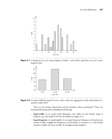
Figure 3.7 A histogram for price using singleton buckets—each bucket represents one price–value/
frequency pair.

25
20

count 15
10

5

0
1–10 11–20 21–30
price ($)

Figure 3.8 An equal-width histogram for price, where values are aggregated so that each bucket has a
uniform width of $10.

“How are the buckets determined and the attribute values partitioned?” There are
several partitioning rules, including the following:

Equal-width: In an equal-width histogram, the width of each bucket range is
uniform (e.g., the width of $10 for the buckets in Figure 3.8).
Equal-frequency (or equal-depth): In an equal-frequency histogram, the buckets are
created so that, roughly, the frequency of each bucket is constant (i.e., each bucket
contains roughly the same number of contiguous data samples).