Page 238 -

#15
2011/6/1
3:19 Page 201
12-ch05-187-242-9780123814791
HAN
5.2 Data Cube Computation Methods 201

with the apex cuboid at the bottom and the base cuboid at the top. In that view, BUC
does bottom-up construction. However, because we adopt the application worldview
where drill-down refers to drilling from the apex cuboid down toward the base cuboid,
the exploration process of BUC is regarded as top-down. BUC’s exploration for the
computation of a 3-D data cube is shown in Figure 5.5.
The BUC algorithm is shown on the next page in Figure 5.6. We first give an expla-
nation of the algorithm and then follow up with an example. Initially, the algorithm is
called with the input relation (set of tuples). BUC aggregates the entire input (line 1)
and writes the resulting total (line 3). (Line 2 is an optimization feature that is discussed
later in our example.) For each dimension d (line 4), the input is partitioned on d (line
6). On return from Partition(), dataCount contains the total number of tuples for each
distinct value of dimension d. Each distinct value of d forms its own partition. Line 8
iterates through each partition. Line 10 tests the partition for minimum support. That
is, if the number of tuples in the partition satisfies (i.e., is ≥) the minimum support,
then the partition becomes the input relation for a recursive call made to BUC, which
computes the iceberg cube on the partitions for dimensions d + 1 to numDims (line 12).
Note that for a full cube (i.e., where minimum support in the having clause is 1), the
minimum support condition is always satisfied. Thus, the recursive call descends one
level deeper into the lattice. On return from the recursive call, we continue with the next
partition for d. After all the partitions have been processed, the entire process is repeated
for each of the remaining dimensions.

Example 5.5 BUC construction of an iceberg cube. Consider the iceberg cube expressed in SQL as
follows:

compute cube iceberg cube as
select A, B, C, D, count(*)
from R
cube by A, B, C, D
having count(*) >= 3

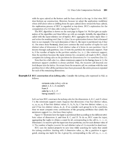
Let’s see how BUC constructs the iceberg cube for the dimensions A, B, C, and D, where
3 is the minimum support count. Suppose that dimension A has four distinct values,
a 1 , a 2 , a 3 , a 4 ; B has four distinct values, b 1 , b 2 , b 3 , b 4 ; C has two distinct values, c 1 , c 2 ;
and D has two distinct values, d 1 , d 2 . If we consider each group-by to be a partition,
then we must compute every combination of the grouping attributes that satisfy the
minimum support (i.e., that have three tuples).
Figure 5.7 illustrates how the input is partitioned first according to the different attri-
bute values of dimension A, and then B, C, and D. To do so, BUC scans the input,
aggregating the tuples to obtain a count for all, corresponding to the cell (∗, ∗ , ∗ , ∗).
Dimension A is used to split the input into four partitions, one for each distinct value of
A. The number of tuples (counts) for each distinct value of A is recorded in dataCount.
BUC uses the Apriori property to save time while searching for tuples that satisfy
the iceberg condition. Starting with A dimension value, a 1 , the a 1 partition is aggre-
gated, creating one tuple for the A group-by, corresponding to the cell (a 1 , ∗ , ∗ , ∗).