Page 240 -

2011/6/1
12-ch05-187-242-9780123814791
#17
3:19 Page 203
HAN
5.2 Data Cube Computation Methods 203

d 1 d 2

a 1 b 1 c 1

c 2

b 2
b 3

b 4

a 2

a 3

a 4

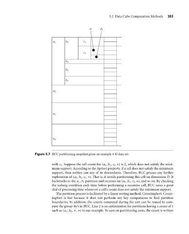
Figure 5.7 BUC partitioning snapshot given an example 4-D data set.

with c 1 . Suppose the cell count for (a 1 , b 1 , c 1 , ∗) is 2, which does not satisfy the mini-
mum support. According to the Apriori property, if a cell does not satisfy the minimum
support, then neither can any of its descendants. Therefore, BUC prunes any further
exploration of (a 1 , b 1 , c 1 , ∗). That is, it avoids partitioning this cell on dimension D. It
backtracks to the a 1 , b 1 partition and recurses on (a 1 , b 1 , c 2 , ∗), and so on. By checking
the iceberg condition each time before performing a recursive call, BUC saves a great
deal of processing time whenever a cell’s count does not satisfy the minimum support.
The partition process is facilitated by a linear sorting method, CountingSort. Count-
ingSort is fast because it does not perform any key comparisons to find partition
boundaries. In addition, the counts computed during the sort can be reused to com-
pute the group-by’s in BUC. Line 2 is an optimization for partitions having a count of 1
such as (a 1 , b 2 , ∗ , ∗) in our example. To save on partitioning costs, the count is written