Page 244 -

HAN
2011/6/1
12-ch05-187-242-9780123814791
3:19 Page 207
#21
5.2 Data Cube Computation Methods 207

Table 5.2 One-Dimensional Aggregates
Dimension count = 1 count ≥ 2
A — a 1 (3), a 2 (2)
B b 2 , b 3 , b 4 b 1 (2)
C c 1 , c 2 , c 4 c 3 (2)
D d 1 , d 2 , d 3 d 4 (2)

Table 5.3 Compressed Base Table: After Star Reduction
A B C D count

a 1 b 1 ∗ ∗ 2
a 1 ∗ ∗ ∗ 1
a 2 ∗ c 3 d 4 2

root:5

a :3 a :2
2
1
b*:1 b :2 b*:2
1

c*:1 c*:2 c :2
3

d*:1 d*:2 d :2
4

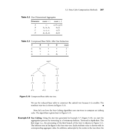
Figure 5.10 Compressed base table star-tree.

We use the reduced base table to construct the cuboid tree because it is smaller. The
resultant star-tree is shown in Figure 5.10.

Now, let’s see how the Star-Cubing algorithm uses star-trees to compute an iceberg
cube. The algorithm is given later in Figure 5.13.

Example 5.8 Star-Cubing. Using the star-tree generated in Example 5.7 (Figure 5.10), we start the
aggregation process by traversing in a bottom-up fashion. Traversal is depth-first. The
first stage (i.e., the processing of the first branch of the tree) is shown in Figure 5.11.
The leftmost tree in the figure is the base star-tree. Each attribute value is shown with its
corresponding aggregate value. In addition, subscripts by the nodes in the tree show the