Page 249 -

12-ch05-187-242-9780123814791
HAN

212 Chapter 5 Data Cube Technology 2011/6/1 3:19 Page 212 #26

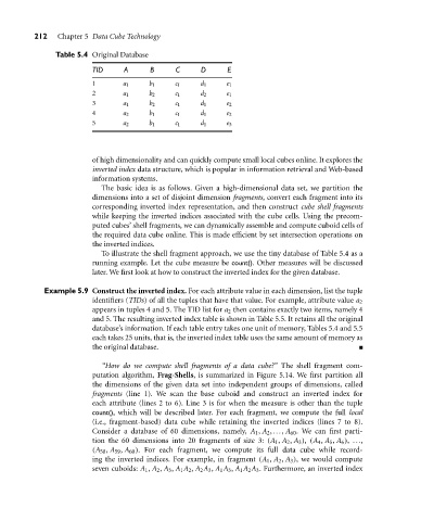
Table 5.4 Original Database

TID A B C D E
1 a 1 b 1 c 1 d 1 e 1
2 a 1 b 2 c 1 d 2 e 1
3 a 1 b 2 c 1 d 1 e 2
4 a 2 b 1 c 1 d 1 e 2
5 a 2 b 1 c 1 d 1 e 3

of high dimensionality and can quickly compute small local cubes online. It explores the
inverted index data structure, which is popular in information retrieval and Web-based
information systems.
The basic idea is as follows. Given a high-dimensional data set, we partition the
dimensions into a set of disjoint dimension fragments, convert each fragment into its
corresponding inverted index representation, and then construct cube shell fragments
while keeping the inverted indices associated with the cube cells. Using the precom-
puted cubes’ shell fragments, we can dynamically assemble and compute cuboid cells of
the required data cube online. This is made efficient by set intersection operations on
the inverted indices.
To illustrate the shell fragment approach, we use the tiny database of Table 5.4 as a
running example. Let the cube measure be count(). Other measures will be discussed
later. We first look at how to construct the inverted index for the given database.

Example 5.9 Construct the inverted index. For each attribute value in each dimension, list the tuple
identifiers (TIDs) of all the tuples that have that value. For example, attribute value a 2
appears in tuples 4 and 5. The TID list for a 2 then contains exactly two items, namely 4
and 5. The resulting inverted index table is shown in Table 5.5. It retains all the original
database’s information. If each table entry takes one unit of memory, Tables 5.4 and 5.5
each takes 25 units, that is, the inverted index table uses the same amount of memory as
the original database.

“How do we compute shell fragments of a data cube?” The shell fragment com-
putation algorithm, Frag-Shells, is summarized in Figure 5.14. We first partition all
the dimensions of the given data set into independent groups of dimensions, called
fragments (line 1). We scan the base cuboid and construct an inverted index for
each attribute (lines 2 to 6). Line 3 is for when the measure is other than the tuple
count(), which will be described later. For each fragment, we compute the full local
(i.e., fragment-based) data cube while retaining the inverted indices (lines 7 to 8).
Consider a database of 60 dimensions, namely, A 1 , A 2 ,..., A 60 . We can first parti-
tion the 60 dimensions into 20 fragments of size 3: (A 1 , A 2 , A 3 ), (A 4 , A 5 , A 6 ), ...,
(A 58 , A 59 , A 60 ). For each fragment, we compute its full data cube while record-
ing the inverted indices. For example, in fragment (A 1 , A 2 , A 3 ), we would compute
seven cuboids: A 1 , A 2 , A 3 , A 1 A 2 , A 2 A 3 , A 1 A 3 , A 1 A 2 A 3 . Furthermore, an inverted index