Page 250 -

12-ch05-187-242-9780123814791
3:19 Page 213
HAN
#27
2011/6/1
5.2 Data Cube Computation Methods 213

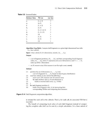
Table 5.5 Inverted Index
Attribute Value TID List List Size

a 1 {1, 2, 3} 3
a 2 {4, 5} 2
b 1 {1, 4, 5} 3
b 2 {2, 3} 2
c 1 {1, 2, 3, 4, 5} 5
d 1 {1, 3, 4, 5} 4
d 2 {2} 1
e 1 {1, 2} 2
e 2 {3, 4} 2
e 3 {5} 1

Algorithm: Frag-Shells. Compute shell fragments on a given high-dimensional base table
(i.e., base cuboid).
Input: A base cuboid, B, of n dimensions, namely, (A 1 ,...,A n ).
Output:
a set of fragment partitions, {P 1 ,...,P k }, and their corresponding (local) fragment
cubes, {S 1 ,..., S k }, where P i represents some set of dimension(s) and P 1 ∪ ... ∪ P k
make up all the n dimensions
an ID measure array if the measure is not the tuple count, count()
Method:
(1) partition the set of dimensions (A 1 ,..., A n ) into
a set of k fragments P 1 ,..., P k (based on data & query distribution)
(2) scan base cuboid, B, once and do the following {
(3) insert each hTID, measurei into ID measure array
(4) for each attribute value a j of each dimension A i
(5) build an inverted index entry: ha j , TIDlisti
(6) }
(7) for each fragment partition P i
(8) build a local fragment cube, S i , by intersecting their
corresponding TIDlists and computing their measures

Figure 5.14 Shell fragment computation algorithm.

is retained for each cell in the cuboids. That is, for each cell, its associated TID list is
recorded.
The benefit of computing local cubes of each shell fragment instead of comput-
ing the complete cube shell can be seen by a simple calculation. For a base cuboid of