Page 251 -

12-ch05-187-242-9780123814791
HAN

214 Chapter 5 Data Cube Technology 2011/6/1 3:19 Page 214 #28

60 dimensions, there are only 7 × 20 = 140 cuboids to be computed according to the
preceding shell fragment partitioning. This is in contrast to the 36,050 cuboids com-
puted for the cube shell of size 3 described earlier! Notice that the above fragment
partitioning is based simply on the grouping of consecutive dimensions. A more desir-
able approach would be to partition based on popular dimension groupings. This
information can be obtained from domain experts or the past history of OLAP queries.
Let’s return to our running example to see how shell fragments are computed.
Example 5.10 Compute shell fragments. Suppose we are to compute the shell fragments of size 3.
We first divide the five dimensions into two fragments, namely (A, B, C) and (D, E).
For each fragment, we compute the full local data cube by intersecting the TID lists in
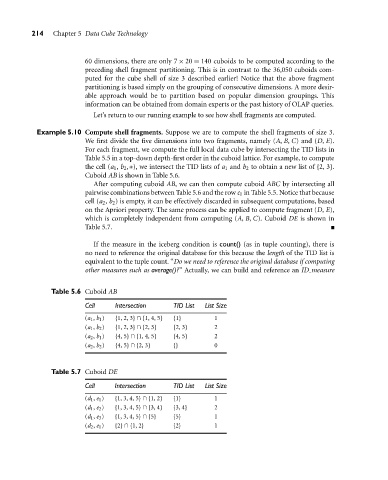
Table 5.5 in a top-down depth-first order in the cuboid lattice. For example, to compute
the cell (a 1 , b 2 ,∗), we intersect the TID lists of a 1 and b 2 to obtain a new list of {2, 3}.
Cuboid AB is shown in Table 5.6.
After computing cuboid AB, we can then compute cuboid ABC by intersecting all
pairwise combinations between Table 5.6 and the row c 1 in Table 5.5. Notice that because
cell (a 2 , b 2 ) is empty, it can be effectively discarded in subsequent computations, based
on the Apriori property. The same process can be applied to compute fragment (D, E),
which is completely independent from computing (A, B, C). Cuboid DE is shown in
Table 5.7.

If the measure in the iceberg condition is count() (as in tuple counting), there is
no need to reference the original database for this because the length of the TID list is
equivalent to the tuple count. “Do we need to reference the original database if computing
other measures such as average()?” Actually, we can build and reference an ID measure

Table 5.6 Cuboid AB
Cell Intersection TID List List Size

(a 1 , b 1 ) {1, 2, 3} ∩ {1, 4, 5} {1} 1
(a 1 , b 2 ) {1, 2, 3} ∩ {2, 3} {2, 3} 2
(a 2 , b 1 ) {4, 5} ∩ {1, 4, 5} {4, 5} 2
(a 2 , b 2 ) {4, 5} ∩ {2, 3} {} 0

Table 5.7 Cuboid DE
Cell Intersection TID List List Size

(d 1 , e 1 ) {1, 3, 4, 5} ∩ {1, 2} {1} 1
(d 1 , e 2 ) {1, 3, 4, 5} ∩ {3, 4} {3, 4} 2
(d 1 , e 3 ) {1, 3, 4, 5} ∩ {5} {5} 1
(d 2 , e 1 ) {2} ∩ {1, 2} {2} 1