Page 243 -

12-ch05-187-242-9780123814791
HAN

206 Chapter 5 Data Cube Technology 2011/6/1 3:19 Page 206 #20

a :30 a :20 a :20 a :20
4
1
2
3
:10 b :10 b :10
b 1 2 3
:5 c :5
c 1 2

d :2 d :3
1
2
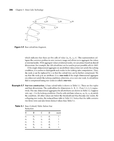
Figure 5.9 Base cuboid tree fragment.

which indicates that there are five cells of value (a 1 , b 1 , c 2 , ∗). This representation col-
lapses the common prefixes to save memory usage and allows us to aggregate the values
at internal nodes. With aggregate values at internal nodes, we can prune based on shared
dimensions. For example, the AB cuboid tree can be used to prune possible cells in ABD.
If the single-dimensional aggregate on an attribute value p does not satisfy the iceberg
condition, it is useless to distinguish such nodes in the iceberg cube computation. Thus,
the node p can be replaced by ∗ so that the cuboid tree can be further compressed. We
say that the node p in an attribute A is a star-node if the single-dimensional aggregate
on p does not satisfy the iceberg condition; otherwise, p is a non-star-node. A cuboid tree
that is compressed using star-nodes is called a star-tree.

Example 5.7 Star-tree construction. A base cuboid table is shown in Table 5.1. There are five tuples
and four dimensions. The cardinalities for dimensions A, B, C, D are 2, 4, 4, 4, respec-
tively. The one-dimensional aggregates for all attributes are shown in Table 5.2. Suppose
min sup = 2 in the iceberg condition. Clearly, only attribute values a 1 , a 2 , b 1 , c 3 , d 4 satisfy
the condition. All other values are below the threshold and thus become star-nodes. By
collapsing star-nodes, the reduced base table is Table 5.3. Notice that the table contains
two fewer rows and also fewer distinct values than Table 5.1.

Table 5.1 Base (Cuboid) Table: Before Star
Reduction
A B C D count

a 1 b 1 c 1 d 1 1
a 1 b 1 c 4 d 3 1
a 1 b 2 c 2 d 2 1
a 2 b 3 c 3 d 4 1
a 2 b 4 c 3 d 4 1