Page 258 - Design and Operation of Heat Exchangers and their Networks

Optimal design of heat exchanger networks 247

(2) Process heat exchangers
Energy balance constraints

_
_
C E,h, j t 0 t 00 Q E, j ¼ 0, C E,c, j t 00 t 0 Q E, j
E,h, j E,h, j E,c, j E,c, j
¼ 0 j ¼ 1, 2, …N E Þ (6.49)
ð
Thermodynamics constraints
t 00 t 0 0, t 0 t 00 0 j ¼ 1, 2, …N E Þ (6.50)
ð
E,c, j E,h, j E,c, j E,h, j
(3) Additional constraints
hxðÞ 0 (6.51)

gxðÞ ¼ 0 (6.52)
Applying a constrained optimization algorithm to the sizing problem (6.38)
under the mapping constraints and the constraints (6.47)–(6.52), we can
determine the optimal heat load of each exchanger in the network together
with the optimal thermal capacity rates of stream splits.

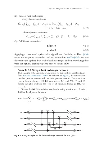
Example 6.3 Sizing a heat exchanger network.
This example is the best network structure for the synthesis problem taken
from Yee and Grossmann (1990). As is shown in Fig. 6.2, the network has
two hot process streams and two cold process streams. There are four
process heat exchangers E1–E4, two mixers M1 and M2. S1 and S2
denote the splits of stream C1. The set of stream is defined as [H1, H2,
C1, C2].
We use the NLP formulation to solve the sizing problem and take the
TAC as the objective function
4 4
X X
TAC xðÞ ¼ 1000A 0:6 + 1200A 0:6 +80Q HU,i + 1000A 0:6 +20Q CU,i
E, j
CU,i
HU,i
j¼1 i¼1
E1 E2 E3
443 293
H1
(30)
E4
423 353
H2
(15)
M2 M1
408 S1 333 C1
(20)
413 S2 303
(40) C2
Fig. 6.2 Sizing example for the heat exchanger network for H2C2_443K.