
Page 265 - Design and Operation of Heat Exchangers and their Networks
P. 265
254 Design and operation of heat exchangers and their networks
180
Q HU,min
160
140
120
Dt m
100
t (°C)
80
60
40
20
Q CU,min
0
0 1000 2000 3000 4000
H (kW)
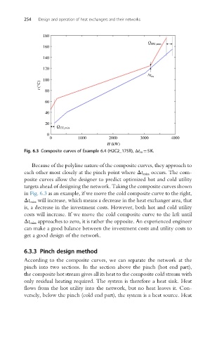
Fig. 6.3 Composite curves of Example 6.4 (H2C2_175R), Δt m ¼5K.
Because of the polyline nature of the composite curves, they approach to
each other most closely at the pinch point where Δt min occurs. The com-
posite curves allow the designer to predict optimized hot and cold utility
targets ahead of designing the network. Taking the composite curves shown
in Fig. 6.3 as an example, if we move the cold composite curve to the right,
Δt min will increase, which means a decrease in the heat exchanger area, that
is, a decrease in the investment costs. However, both hot and cold utility
costs will increase. If we move the cold composite curve to the left until
Δt min approaches to zero, it is rather the opposite. An experienced engineer
can make a good balance between the investment costs and utility costs to
get a good design of the network.
6.3.3 Pinch design method
According to the composite curves, we can separate the network at the
pinch into two sections. In the section above the pinch (hot end part),
the composite hot stream gives all its heat to the composite cold stream with
only residual heating required. The system is therefore a heat sink. Heat
flows from the hot utility into the network, but no heat leaves it. Con-
versely, below the pinch (cold end part), the system is a heat source. Heat