Page 277 - Design and Operation of Heat Exchangers and their Networks

Optimal design of heat exchanger networks 263

180

160
Q HU,min
140

120
t (°C)

100
Dt m
80 Q CU,min

60
Dt m
40
0 10,000 20,000 30,000 40,000
H (kW)
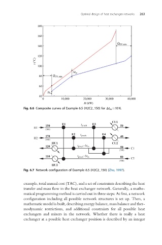
Fig. 6.6 Composite curves of Example 6.5 (H2C2_150) for Δt m ¼10K.

CU1
E1 t E3
150 pinch 50
H1
(200)
E2 t E4
170 pinch 40
H2
(100)
HU1 CU2
120 t pinch –Dt m 50 C1
(300)
110 t pinch –Dt m 80
C2
(500)
HU2
Fig. 6.7 Network configuration of Example 6.5 (H2C2_150) (Zhu, 1997).

example, total annual cost (TAC), and a set of constraints describing the heat
transfer and mass flow in the heat exchanger network. Generally, a mathe-
matical programming method is carried out in three steps: At first, a network
configuration including all possible network structures is set up. Then, a
mathematic model is built, describing energy balance, mass balance and ther-
modynamic restrictions, and additional constraints for all possible heat
exchangers and mixers in the network. Whether there is really a heat
exchanger at a possible heat exchanger position is described by an integer