Page 274 - Design and Operation of Heat Exchangers and their Networks

Optimal design of heat exchanger networks 261

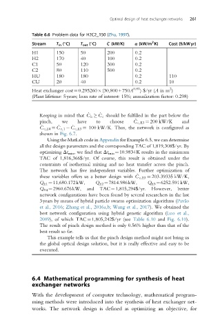
Table 6.6 Problem data for H2C2_150 (Zhu, 1997).
2
_
Stream T in (°C) T out (°C) C (kW/K) α (kW/m K) Cost ($/kWyr)
H1 150 50 200 0.2
H2 170 40 100 0.2
C1 50 120 300 0.2
C2 80 110 500 0.2
HU 180 180 0.2 110
CU 20 40 0.2 10
0.81 2
Heat exchanger cost¼0.295260 (30,800+750A ) $/yr (A in m )
(Plant lifetime: 5years; loan rate of interest: 15%; annualization factor: 0.298)

_
_
Keeping in mind that C h C c should be fulfilled in the part below the
_
pinch, we have to choose C c,E3 ¼ 200 kW/K and
_
_
_
C c,E4 ¼ C c,1 C c,E3 ¼ 100 kW/K. Thus, the network is configured as
shown in Fig. 6.7.
Using the MatLab code in Appendix for Example 6.5, we can determine
all the design parameters and the corresponding TAC of 1,819,308$/yr. By
optimizing Δt min , we find that Δt min ¼10.9834K results in the minimum
TAC of 1,816,366$/yr. Of course, this result is obtained under the
constraints of isothermal mixing and no heat transfer across the pinch.
The network has five independent variables. Further optimization of
_
these variables offers us a better design with C c,E3 ¼ 203:39335 kW/K,
Q E1 ¼11,680.172kW, Q E2 ¼7814.986kW, Q E3 ¼6252.591kW,
Q E4 ¼2960.676kW, and TAC¼1,815,294$/yr. However, better
network configurations have been found by several researchers in the last
3years by means of hybrid particle swarm optimization algorithms (Pava ˜o
et al., 2016; Zhang et al., 2016a,b; Wang et al., 2017). We obtained the
best network configuration using hybrid genetic algorithm (Luo et al.,
2009), of which TAC¼1,805,242$/yr (see Table 6.10 and Fig. 6.10).
The result of pinch design method is only 0.56% higher than that of the
best result so far.
This example tells us that the pinch design method might not bring us
the global optical design solution, but it is really effective and easy to be
executed.

6.4 Mathematical programming for synthesis of heat
exchanger networks

With the development of computer technology, mathematical program-
ming methods were introduced into the synthesis of heat exchanger net-
works. The network design is defined as optimizing an objective, for