Page 222 - Design for Six Sigma a Roadmap for Product Development

194 Chapter Six

In this case we have f 3 ● (f 1 , f 2 ) f 3 (
2 f i (M, DP i ), DP 3 ) f 3 (M 3 ,DP 3 ).
i 1
The transfer function is given as

{ }
A 11 0 0 0 DP 1
FR 1 β 1 DP 2
FR 2 0 A 22 0 0 β 2 DP 3 error (noise
{ } [ 0 0 factors) (6.4)
FR 3 A 33 β 1β 3 β 2β 3 ] M 1
M 2
A 11 0 0 DP 1 β 1 0
M 1
0 A 22 DP 2 0 β 2 ] { M 2} error (noise
[ 0 0 A 33 ]{ } [ β 1β 3 β 2β 3 factors) (6.5)
DP 3
with the constraint M 3 FR 1 FR 2 .
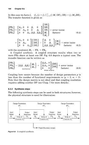
4. Coupled synthesis. A coupled structure results when two or
more FRs share at least one DP. Fig. 6.6 depicts a typical case. The
transfer function can be written as
{ } M 1 } [ ] {DP} error (noise
β 3 A 11 0
DP
FR 1
1
β 3 A 21 0
FR 2 [β 1β 3 β 2β 3 ]
FR 3 ideal function { M 2 0 0 3 factors) (6.6)
design mapping
Coupling here occurs because the number of design parameters p is
less than the number of functional requirements m (p 2, m 3).
Note that the design matrix is not ideal and that coupling resolution
requires adding another DP (see Chap. 7 for more details).

6.3.3 Synthesis steps
The following synthesis steps can be used in both structures; however,
the physical structure is used for illustration:

Design Parameters Design Parameters Design Parameters
DP 1 DP 2 DP 3

Input Output Input Output Input Output
Signal Response Signal Response Signal Response
M 1 Entity of FR 1 M 2 Entity of FR 2 M 3 Entity of FR 3
Function #1 Function #2 Function #3

Project Boundary (scope)
Figure 6.6 A coupled synthesis.