Page 229 - Design for Six Sigma a Roadmap for Product Development

200 Chapter Six

Ohm laws and digital logic circuit design and to derive their project
FRs. The transfer functions obtained through this source are very
dependent on the team’s understanding and competency with their
design and the discipline of knowledge it represents (engineering,
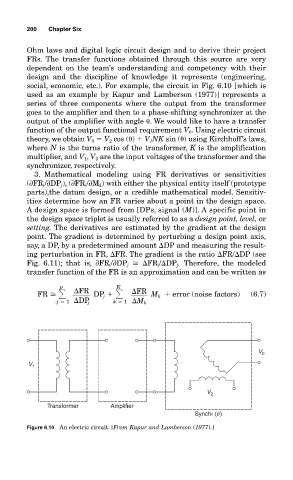
social, economic, etc.). For example, the circuit in Fig. 6.10 [which is
used as an example by Kapur and Lamberson (1977)] represents a
series of three components where the output from the transformer
goes to the amplifier and then to a phase-shifting synchronizer at the
output of the amplifier with angle . We would like to have a transfer
function of the output functional requirement V 0 . Using electric circuit
theory, we obtain V 0 V 2 cos ( ) V 1 NK sin ( ) using Kirchhoff’s laws,
where N is the turns ratio of the transformer, K is the amplification
multiplier, and V 1 , V 2 are the input voltages of the transformer and the
synchronizer, respectively.
3. Mathematical modeling using FR derivatives or sensitivities
(∂FR i /∂DP j ), (∂FR i /∂M k ) with either the physical entity itself (prototype
parts),the datum design, or a credible mathematical model. Sensitiv-
ities determine how an FR varies about a point in the design space.
A design space is formed from [DPs, signal (M)]. A specific point in
the design space triplet is usually referred to as a design point, level, or
setting. The derivatives are estimated by the gradient at the design
point. The gradient is determined by perturbing a design point axis,
say, a DP, by a predetermined amount DP and measuring the result-
ing perturbation in FR, FR. The gradient is the ratio FR/ DP (see
Fig. 6.11); that is, ∂FR i /∂DP j FR i / DP j . Therefore, the modeled
transfer function of the FR is an approximation and can be written as

p K
FR
FR
FR
DP j
M k error (noise factors) (6.7)
j 1 DP j k 1 M k

V 0
V 1

V 2

Transformer Amplifier
Synchr ( )
Figure 6.10 An electric circuit. [From Kapur and Lamberson (1977).]