Page 231 - Design for Six Sigma a Roadmap for Product Development

202 Chapter Six

where x stands for all the variables affecting the FR (signal, DPs, and
noise) and L is the number of noise factors. The variance of the vari-
ables can be estimated from historical data or assessed. The worst-case
scenario is usually used. Notice that the sensitivities are designed in
by the team as they decide the DPs and the physical structure while
the parameter variables are controlled by operations. This equation
stresses the fact that a Six Sigma–capable design needs the contri-
bution of both design and operations. The design experts in the team
can use their expertise to modify the sensitivities and the operation
members, the variances. We view this equation as the equation that
captures the concurrent engineering concept in mathematical terms.
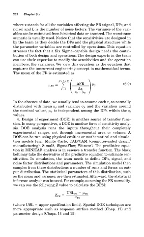
The mean of the FR is estimated as

P L K
FR
FR
j (6.9)
j 1 x j
x j
j
In the absence of data, we usually tend to assume each x j as normally
distributed with mean j and variance j , and the variation around
the nominal values, j , is independent among the DPs within the x j
values.
4. Design of experiment (DOE) is another source of transfer func-
tion. In many perspectives, a DOE is another form of sensitivity analy-
sis. DOE analysis runs the inputs throughout their completely
experimental ranges, not through incremental area or volume. A
DOE can be run using physical entities or mathematical and simula-
tion models [e.g., Monte Carlo, CAD/CAM (computer-aided design/
manufacturing), Simul8, SigmaFlow, Witness]. The predictive equa-
tion in MINITAB analysis is in essence a transfer function. The black
belt may take the derivative of the predictive equation to estimate sen-
sitivities. In simulation, the team needs to define DPs, signal, and
noise factor distributions and parameters. The simulation model then
samples from these distributions a number of runs and forms an out-
put distribution. The statistical parameters of this distribution, such
as the mean and variance, are then estimated. Afterward, the statistical
inference analysis can be used. For example, assuming the FR normality,
we can use the following Z value to calculate the DPM:

USL FR FR
Z FR
FR
(where USL upper specification limit). Special DOE techniques are
more appropriate such as response surface method (Chap. 17) and
parameter design (Chaps. 14 and 15).