Page 444 - Design for Six Sigma for Service (Six SIGMA Operational Methods)

402 Chapter Eleven

f(y)

Distribution
with smaller s

Distribution
with larger s
y
Figure 11.4 Normal Probability Density Curve

For the normal distribution,
E(y) = m and Var(y) = s 2
2
A normal random variable y with E(y) = m and Var(y) = s is denoted by
2
N(m, s ). The probability density function f(y) displays a bell-shaped curve
as illustrated by Fig. 11.4. The distribution is centered at m, and the smaller
s results in a tighter curve and vice versa.

An important special case of the normal distribution is the standard normal
2
distribution. In the standard normal distribution, m = 0 and s = 1. The
standard normal random variable is often denoted by z ~ N(0, 1). The
standard normal distribution table is mainly used to calculate probabilities
for all kinds of normal distributions.
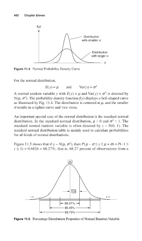
Figure 11.5 shows that if y ~ N(m, s ), then P(m − s ≤ y ≤ m + s) = P(–1 ≤
2
z ≤ 1) = 0.6826 = 68.27%; that is, 68.27 percent of observations from a

m

1s
− ∞ + ∞
68.27%
95.45%
99.73%
Figure 11.5 Percentage Distribution Properties of Normal Random Variable