Page 446 - Design for Six Sigma for Service (Six SIGMA Operational Methods)

404 Chapter Eleven

This binomial distribution is often denoted by y ~ B(n, p). The following are
examples of binomial random variables:
1. The number of defective parts, y, in a lot of n parts in a sequential
quality inspection
2. The number of positive customer responses, y, in a survey involving n
customers

Poisson Distribution
The Poisson probability distribution provides a model for the probability of
occurrence of the number of rare events that happen in a unit of time, area,
volume, and so on. Actually, the Poisson distribution is an extreme case of
the binomial distribution, where n is very large and p is very small. That is,
the probability of a rare event occurrence p = P(S) is very small, but the
number of trials n is very large.

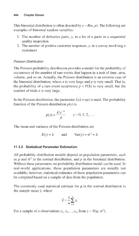
In the Poisson distribution, the parameter l(l = np) is used. The probability
function of the Poisson distribution p(y) is

l y −l
e
py() = y = 0, 1, 2, . . .
y!
The mean and variance of the Poisson distribution are
E(y) =λ and Var(y) = s = l
2

11.3.2 Statistical Parameter Estimation
All probability distribution models depend on population parameters, such
2
as m and s in the normal distribution, and p in the binomial distribution.
Without these parameters, no probability distribution model can be used. In
real-world applications, these population parameters are usually not
available; however, statistical estimates of these population parameters can
be computed based on a sample of data from the population.

The commonly used statistical estimate for m in the normal distribution is
_
the sample mean y, where
n
1
y = ∑ y
n i=1 i
2
For a sample of n observations y , y ,…,y , from y ~ N(m, s ).
n
1
2