Page 231 - Determinants and Their Applications in Mathematical Physics

216 5. Further Determinant Theory

1 −4x 10x 2
1 −3x 6x 2 −10x 2
1 −2x 3x 2 −4x 3 5x 4
1 −x x 2 −x 3 x 4 −x 5
(5.6.13)
1 α 0 α 1 α 2 α 3 α 4 α 5
1 −x α 1 α 2 α 3 α 4 α 5 α 6
−2x x 2 α 2 α 3 α 4 α 5 α 6
3x 2 −x 3 α 3 α 4 α 5 α 6

66
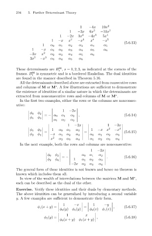
These determinants are B , s =1, 2, 3, as indicated at the corners of the
s
frames. B 66 is symmetric and is a bordered Hankelian. The dual identities
1
are found in the manner described in Theorem 5.16.
All the determinants described above are extracted from consecutive rows
and columns of M or M . A few illustrations are sufficient to demonstrate
∗
the existence of identities of a similar nature in which the determinants are
extracted from nonconsecutive rows and columns of M or M .
∗
In the first two examples, either the rows or the columns are nonconsec-
utive:

1 −2x
φ 0

= − α 0 α 1
φ 2 , (5.6.14)
φ 1 φ 3
α 2
α 1 α 2 α 3

1 1

−2x −3x
2
1 1 −x x 3

φ 1 α 0 α 1 α 2 −x

φ 3 .(5.6.15)
=
=
φ 2 φ 4 −xα 1 α 2 α 3 α 0 α 1 α 2 α 3

x α 2 α 3 α 4 α 1 α 2 α 3 α 4
2
In the next example, both the rows and columns are nonconsecutive:
1

−2x

φ 0 α 0 α 1

α 2
φ 2
. (5.6.16)
1
= −
φ 2 φ 4 α 1 α 2 α 3

−2xα 2 α 3 α 4
The general form of these identities is not known and hence no theorem is
known which includes them all.
In view of the wealth of interrelations between the matrices M and M ,
∗
each can be described as the dual of the other.
Exercise. Verify these identities and their duals by elementary methods.
The above identities can be generalized by introducing a second variable
y. A few examples are sufficient to demonstrate their form.

1 −x 1 −y

φ 1 (x + y)= = , (5.6.17)
φ 0 (y) φ 1 (y) φ 0 (x) φ 1 (x)

1 x
φ 1 (y)= , (5.6.18)
φ 0 (x + y) φ 1 (x + y)