Page 248 - Digital Analysis of Remotely Sensed Imagery

212 Cha pte r S i x

extremely bright or dark objects are likely to occupy a wide range of
DNs. Consequently, there is an imbalance in the number of pixels at a
given DN (Fig. 6.8a). This imbalance represents an inefficient alloca-
tion of pixel DNs. Intuitively, the predominant pixels should be repre-
sented in a wider range of DNs so that the subtle spectral variations
among them can be readily differentiated. This imbalance is ideally
remedied through histogram equalization. This nonlinear contrast
manipulation technique achieves an enhanced contrast at the expense
of losing minor details in the input image. In the output image, distri-
bution of pixels is roughly equalized through aggregation of minority
pixels of a similar gray level into one value. Therefore, the output
image always contains fewer levels of DN than the raw image. The
DN range vacated from the aggregation is used by pixels of a pre-
dominant quantity. In this way, the spectral distance or disparity
between any two adjoining DNs is artificially broadened. Since the
number of pixels at a given DN varies widely, the aggregated fre-
quency is rarely equalized no matter how differently individual fre-
quencies in the histogram are combined. Instead, the discrepancy
between the maximum and minimum number of pixels at different
DNs is reduced in comparison to the raw distribution (Fig. 6.8b).
The undertaking of histogram equalization requires a few specifi-
cations, including the number of gray levels in the output image.
Then the probability for each pixel to occur in one of these levels is
calculated. The calculation is illustrated using a hypothetical image
of 7 × 8 pixels recorded at 4 bits (Fig. 6.8). Most of the 56 pixels have a
DN centered at 5 and 13 (Fig. 6.8a). The first step in performing histo-
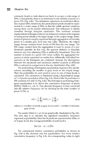
gram equalization is to derive the cumulative frequency of pixels
Σf(DN) (Table 6.1, col. 3). This absolute frequency is then converted
j
into the relative frequency c(k) by dividing by the total number of
pixels N (56), or

k
k
ck() = 1 ∑ fDN ) = 1 ∑ n (6.6)
(
N j N j
j=0 j=0
where n = number of pixels at gray level jand k = number of discrete
j
gray levels.
The results (Table 6.1, col. 4) are graphically illustrated in Fig. 6.8c.
The next step is to calculate the equalized cumulative frequency
expressed as probability. Since the 56 pixels are represented in 4 bits, or
at 16 gray levels, the average probability of each level is

56/(16 − 1) = 6.25%
The constructed relative cumulative probability as shown in
Fig. 6.8d is the decision rule for equalization. For every relative
cumulative frequency in Fig. 6.8c, its corresponding value in right